Basics and Definitions
Before studying directed technological change, it is useful to clarify the difference between factor-augmenting and factor-biased technological changes, which are sometimes confused in the literature.
For this purpose and for much of the analysis in this chapter, we assume that the production side of the economy can be represented by an aggregate production function,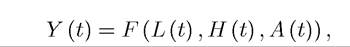
567
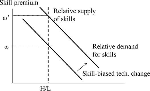
FIGURE 15.2. The effect of H-biased technological change on relative demand and relative factor prices.
where L (t) is labor, and H (t) denotes another factor of production, which could be skilled labor, capital, land or some intermediate goods, and A (t) represents technology. Without loss of generality imagine that ∂F∕∂A > 0, so a greater level of A corresponds to “better technology”. Recall that technological change is L-augmenting if
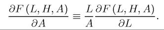
This is clearly equivalent to the production function taking the more special form, F (AL, H). In the case where L corresponds to labor and H to capital, this is also equivalent to Harrod- neutral technological change. Conversely, H-augmenting technological change is defined similarly, and corresponds to the production function taking the special form F (L, AH).
Though often equated with factor-augmenting changes, the concept of factor-biased technological change is very different. We say that technological change change is L-biased, if it increases the relative marginal product of factor L compared to factor H. Mathematically, this corresponds to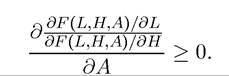
Put differently, biased technological change shifts out the relative demand curve for a factor, so that its relative marginal product (relative price) increases at given factor proportions (i.e., given relative quantity of factors).
Conversely, technological change is H-biased if this inequality holds in reverse. Figure 15.2 plots the effect of an H-biased (skill-biased) technological change on the relative demand for factor H and on its relative price, the skill premium.These concepts can be further clarified using the constant elasticity of substitution (CES) production function, which we will use for the rest of this chapter. The CES production function takes the form  where Al (t) and A∏ (t) are two separate technology terms, the γis determine the importance of the two factors in the production function, and
 Finally, σ ∈ (0, ∞) is
the elasticity of substitution between the two factors. When σ = ∞, the two factors are perfect substitutes, and the production function is linear. When σ = 1, the production function is Cobb-Douglas, and when σ = 0, there is no substitution between the two factors, and the production function is Leontieff. When σ > 1, we refer to the factors as “gross substitutes,” and when σ < 1, we refer to them as “gross complements”. While there are multiple definitions of complementarity in the microeconomics literature, this terminology is useful to distinguish the two cases in which σ < 1 and σ > 1, which will have very different implications in the current context.
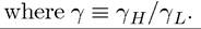
Clearly, by construction, Al (t) is L-augmenting, while Ah (t) is H-augmenting. Interestingly, whether technological change that is L-augmenting (or H-augmenting) is L-biased or H-biased depends on the elasticity of substitution, σ. Let us first calculate the relative marginal product of the two factors (see Exercise 15.1):
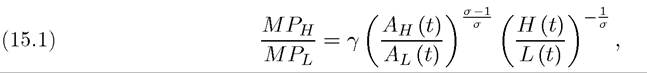
 The relative marginal product of H is decreasing in its relative abundance, H (t) /L (t). This is simply the consequence of the usual substitution effect, leading to a negative relationship between relative supplies and relative marginal products (or prices) and thus to a downward-sloping relative demand curve (see Figure 15.3).
The intuition for why, when σ < 1, H-augmenting technical change is L-biased is simple but important: with gross complementarity (σ < 1), an increase in the productivity of H 569
increases the demand for labor, L, by more than the demand for H. As a result, the marginal product of labor increases by more than the marginal product of H. This can be seen most clearly in the extreme case where σ → 0, so that the two factors become Leontieff. In this case, starting from a situation in which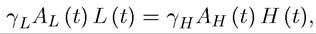 a small increase in
Ah (t) will create an “excess of the services” of the H factor (and thus “excess demand” for L), and the price of factor H will fall to 0.
I have so far de fined the meaning of H-biased and L-biased technological changes. It is also useful to define two concepts that will play a major role in the remainder of this chapter. There is weak equilibrium bias of technology if an increase in the relative supply of H, H/L, induces technological change biased towards H.
Mathematically, this is equivalent to: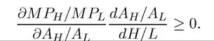
From (15.1), it is clear that this condition will hold if
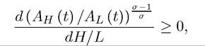
so that in response to the change in relative supplies Ah (t) /Al (t) changes in a direction that is biased towards the factor that has become more abundant.
On the other hand, there is strong equilibrium bias if an increase in H/L induces a sufficiently large change in the bias of technology so that the marginal product of H relative to that of L increases following the change in factor supplies. Mathematically, this is equivalent to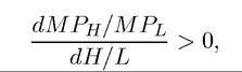
where I now use a strict inequality to distinguish strong equilibrium bias from the case in which relative marginal products are independent of relative supplies (e.g., because factors are perfect substitutes). These equations make it clear that the major difference between weak and strong equilibrium bias is whether the relative marginal product of the two factors are evaluated at the initial relative supplies (in the case of weak bias) or at the new relative supplies (in the case of strong bias). Consequently, strong equilibrium bias is a much more demanding concept than weak equilibrium bias.
15.3.