Baseline Model of Directed Technological Change

In this section, we present the baseline model of directed technological change, which uses the expanding varieties model of endogenous technological change and the lab equip­ment specification of the innovation possibilities frontier.

externalities. Section 15.4 will consider a model of directed technological with change knowl­edge spillovers. Exercise 15.19 shows that all of the results presented here generalize to a model of Schumpeterian growth, thus the assumption of expanding varieties is only adopted for convenience.

The baseline economy has a constant supply of two factors, L and H, and admits a representative household with the standard CRRA preferences given by

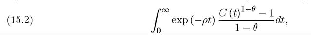
where, as usual, p > 0. The supply side is represented by an aggregate production function combining the outputs of two intermediate sectors with a constant elasticity of substitution: where Yl (t) and Yh (t) denote the outputs of two intermediate goods. As the indices indicate, the first is L-intensive, while the second is H -intensive. The parameter ε ∈ [0, ∞) is the elasticity of substitution between these two intermediate goods. The assumption that (15.3) features a constant elasticity of substitution simplifies the analysis but is not crucial for the results. How relaxing this assumption affects the results is discussed at the end of this chapter.

The resource constraint of the economy at time t takes the form

(15.4) C (t) + X (t) + Z (t) ≤ Y (t),

where, as before, X (t) denotes total spending on machines and Z (t) is aggregate R&D spending.

The two intermediate goods are produced competitively with the following production functions:

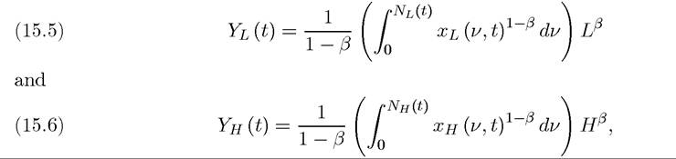
where xl (ν, t) and xh (ν, t) denote the quantities of the different types of machines (used in the production of one or the other intermediate good) and β ∈ (0,1).^[XXIX] These machines are again assumed to depreciate after use. The parallel between these production functions and the aggregate production function of the economy in the baseline expanding product varieties model of Chapter 13 is obvious. There are two important differences, however. First, these are now production functions for intermediate goods rather than the final good. Second, the two production functions (15.5) and (15.6) use different types of machines. The range of machines complementing labor, L, is [0,Nl (t)], while the range of machines complementing factor H is [0,Nh (t)].

Again as in Chapter 13, we assume that all machines in both sectors are supplied by monopolists that have a fully-enforced perpetual patent on the machines. We denote the prices charged by these monopolists at time t by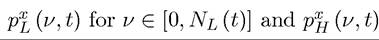for

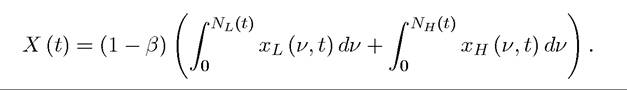
Once invented, each machine can be produced at the fixed marginal cost ψ in terms of the final good, which we again normalize to ψ ? 1 — β. This implies that total resources devoted to machine production at time t are

The innovation possibilities frontier is assumed to take a form similar to the lab equipment specification in Chapter 13:

where Zl (t) is R&D expenditure directed at discovering new labor-augmenting machines at time t, while Zh (t) is R&D expenditure directed at discovering H -augmenting machines.

The value of a monopolist that discovers one of these machines is again given by the standard formula for the present discounted value of profits:

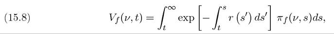
whereagain denotes instantaneous profits for f = L

or H, and r (t) is the market interest rate at time t. Once again, it is sometimes more convenient to work with the Hamilton-Jacobi-Bellman version of this value function, which takes the form:

(15.9)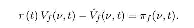

Throughout, we normalize the price of the final good at every instant to 1, which is equivalent to setting the ideal price index of the two intermediates equal to one, i.e., where pl (t) is the price index of Yl at time t and p∏ (t) is the price of Y∏. We also denote the factor prices by Wl (t) and w∏ (t).

15.3.1. Characterization of Equilibrium. An allocation in this economy is de­fined by the following objects: time paths of consumption levels, aggregate spend-

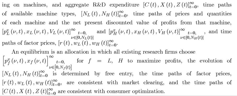
To characterize the (unique) equilibrium, let us first consider the maximization problem of producers in the two sectors. Since machines depreciate fully after use, these maximization problems are static and can be written as

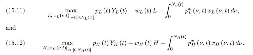
The main difference from the maximization problem facing final good producers in Chapter 13 is the presence of prices p_k (t) and p∏ (t), which reflect the fact that these sectors pro­duce intermediate goods, whereas factor and machine prices are expressed in terms of the numeraire, the final good.

These two maximization problems immediately imply the following demand for machines in the two sectors:

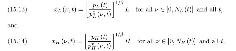
Similar to the demands for machines in Chapter 13, these are iso-elastic, so the maximization of the net present discounted value of profits implies that each monopolist should set a constant markup over marginal cost and thus a price of

573

Substituting these prices into (15.13) and (15.14), we obtain

and

Since these quantities do not depend on the identity of the machine, only on the sector that is being served, profits are also independent of the machine type. In particular, we have

This implies that the net present discounted values of monopolists only depend on which sector they are supplying and can be denoted by Vr (t) and V∏ (t).

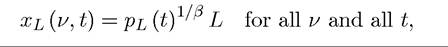
Next, combining these with (15.5) and (15.6), we obtain the derived production functions for the two intermediate goods: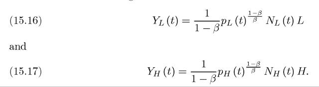

These derived production functions are similar to (13.12) in Chapter 13, except for the presence of the price terms.

Finally, the prices of the two intermediate goods are derived from the marginal product conditions of the final good technology, (15.3), which imply

is the (derived) elasticity of substitution between the two factors. The first line of this expression simply defines p (t) as the relative price between the two intermediate goods and uses the fact that the ratio of the marginal productivities of the two intermediate goods must be equal to this relative price.

574

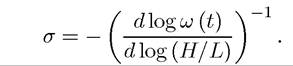
Using the latter equation, we can also calculate the relative factor prices in this economy as:

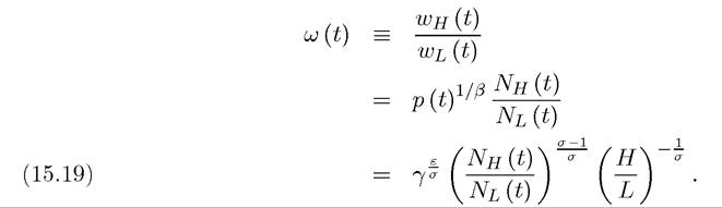
The first line of (15.19) defines ω (t) as the relative wage of factor H compared to factor L. The second line uses the definition of marginal product combined with (15.16) and (15.17), and the third line uses (15.18). We refer to σ as the (derived) elasticity of substitution between the two factors, since it is exactly equal to

To complete the description of equilibrium in the technology side, we need to impose the

following free entry conditions:

and

Finally, the consumer side is characterized by the same necessary conditions as usual:

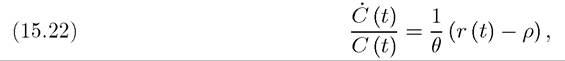
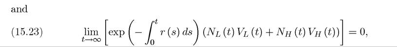
this economy.

We are now in a position to characterize a balanced growth path (BGP) equilibrium. Let us define the BGP equilibrium to be one in which consumption grows at the constant rate, g*, and the relative price p (t) is constant. From (15.10) this implies that pl (t) and ðí (t)

are also constant.

Let Vl and V∏ be the BGP net present discounted values of new innovations in the two sectors. Then (15.9) implies that

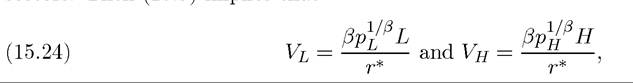
where r* is the BGP interest rate, while pl and p∣∕ are the BGP prices of the two intermediate goods.

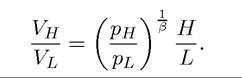
above, the greater is Vh relative to VL, the greater are the incentives to develop H-augmenting machines, Nh, rather than Nl- Taking the ratio of these two expressions, we obtain

This expression highlights the two effects on the direction of technological change dis­cussed in Section 15.1.

(1) The price effect manifests itself because Vh/Vl is increasing in ðí/pl- The greater is this relative price, the greater are the incentives to invent technologies complement­ing the H factor. Since goods produced by relatively scarce factors will be relatively more expensive, the price effect tends to favor technologies complementing scarce factors.

(2) The market size effect is a consequence of the fact that V∏/Vl is increasing in H∕L. The market for a technology is the workers (or the other factors) that will be using and working with this technology. Consequently, an increase in the supply of a factor translates into a greater market for the technology complementing that factor. The market size effect encourages innovation for the more abundant factor.

The above discussion is incomplete, however, since prices are endogenous. Combining (15.24) together with (15.18), we can eliminate relative prices and obtain the relative prof­itability of the technologies as:

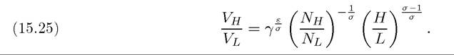
Note for future reference that an increase in the relative factor supply, H∕L, will increase Vh/Vl as long as σ > 1 and it will reduce it if σ < 1. This shows that the elasticity of substitution between the factors, σ, regulates whether the price effect dominates the market size effect. Since σ is not a primitive, but a derived parameter, we would like to know when it is greater than 1. It is straightforward to check that

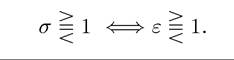
So the two factors will be gross substitutes when the two intermediate goods are gross sub­stitutes in the production of the final good.

Next, using the two free entry conditions (15.20) and (15.21), and assuming that both of them hold as equalities, we obtain the following BGP “technology market clearing” condition:

Combining this with (15.25), we obtain the following BGP ratio of relative technologies

576

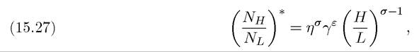
where η ? η∣_l/n_L and the *'s denote that this expression refers to the BGP value. The notable feature here is that relative productivities are determined by the innovation possibilities frontier and the relative supply of the two factors. In this sense, this model totally endogenizes technology. Equation (15.27) contains most of the economics of directed technology. However, before discussing this, it is useful to characterize the BGP growth rate of the economy. This is done in the next proposition:

PROPOSITION 15.1. Consider the directed technological change model described above. Suppose that

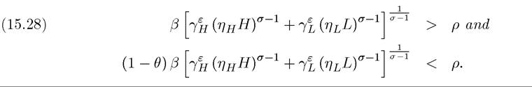
Then there exists a unique BGP equilibrium in which the relative technologies are given by (15.27), and consumption and output grow at the rate

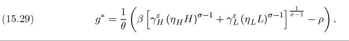
Proof. The derivation of (15.29) is provided by the argument preceding the proposition. Exercise 15.2 asks you to check that condition (15.28) ensures that free entry conditions (15.20) and (15.21) must hold, to verify that this is the unique relative equilibrium technology, to calculate the BGP equilibrium growth rate and to verify that the transversality condition is satisfied. ?

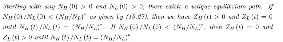
It can also be verified that there are simple transitional dynamics in this economy whereby starting with technology levels N∣∣ (0) and Nl (0), there always exists a unique equilibrium path and it involves the economy monotonically converging to the BGP equilibrium of Propo­sition 15.1. This is stated in the next proposition:

PROPOSITION 15.2. Consider the directed technological change model described above.

Proof. See Exercise 15.3. ?

More interesting than the aggregate growth rate and the transitional dynamics behavior of the economy are the results concerning the direction of technological change and its effects on relative factor prices. These are studied in the next subsection.

15.3.2. Directed Technological Change and Factor Prices. Let us start by study­ing (15.27). This equation implies that, in BGP, there is a positive relationship between the

This immediately establishes the following weak equilibrium bias result:

PROPOSITION 15.3. Consider the directed technological change model described above. There is always weak equilibrium (relative) bias in the sense that an increase in H/L always induces relatively H -biased technological change.

Recall that weak bias was defined in Section 15.2 with a weak inequality, so that the proposition is also correct when σ = 1, even though in this case it can be verified easily from

Proposition 15.3 is the basis of the discussion about induced biased technological change in Section 15.1, and already gives us a range of insights about how changes in the relative supplies of skilled workers may be at the root of the skill-biased technological change. These implications are further discussed in the next subsection.

The results of this proposition reflect the strength of the market size effect discussed above. Recall that the price effect creates a force favoring factors that become relatively scarce. In contrast, the market size effect, which is related to the non-rivalry of ideas discussed in Chapter 12, suggests that technologies should change in a way that favors factors that are becoming relatively abundant. Proposition 15.3 shows that the market size effect always dominates the price effect.

Proposition 15.3 is only informative about the direction of the induced technological change, but does not specify whether this induced effect will be strong enough to make the endogenous-technology relative demand curve for factors upward-sloping. Recall that in basic producer theory, all demand curves, and thus relative demand curves, are downward-sloping as well. However, as hinted in Section 15.1, directed technological change can lead to the 578

seemingly paradoxical result that relative demand curves can be upward-sloping once the endogeneity of technology is taken into account. To obtain this result, let us substitute for 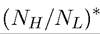from (15.27) into the expression for the relative wage given technologies, (15.19), and obtain the following BGP relative factor price ratio (see Exercise 15.4):

Inspection of this equation immediately establishes conditions for strong equilibrium (relative) bias.

PROPOSITION 15.4. Consider the directed technological change model described above. Then if σ > 2, there is strong equilibrium (relative) bias in the sense that an increase in H/L raises the relative marginal product and the relative wage of the factor H compared to factor L.

Figure 15.3 illustrates the results of Propositions 15.3 and 15.4, referring to H as skilled labor and L as unskilled labor as in the first application discussed in Section 15.1.

Figure 15.3. The relationship between the relative supply of skills and the skill premium in the model of directed technical change.

The curve marked with CT corresponds to the constant-technology relative demand from equation (15.19). It is always downward-sloping because it holds the relative technologies, Nh/Nl, constant, and thus only features the usual substitution effect. The fact that this 579

curve is downward-sloping follows from basic producer theory. The curve marked as ETi applies when technology is endogenous, but the condition in Proposition 15.4, that σ > 2, is not satisfied. We know from Proposition 15.3 that even in this case an increase in H/L will induce skill-biased (H-biased) technological change. This implies that when H/L is higher than its initial level, the induced-technology effect will shift the constant-technology demand curve CT to the right (i.e., as technology changes, it will be another CT curve, above the original one, that will apply). When it is below, the same effect will shift CT to the left. Consequently, the locus of points that the endogenous-technology demand, ETi, is shallower than CT. [This can be also verified comparing the relative demand functions with constant and endogenous technology, (15.19) and (15.30), and noting that σ — 2 is never less than — 1∕σ]. There is an obvious analogy between this result and Samuelson’s LeChatelier principle, which states that long-run demand curves, which apply when all factors can adjust, must be more elastic than the short-run demand curves which hold some factors constant. We can think of the endogenous-technology demand curve as adjusting the “factors of production” corresponding to technology. However, the analogy is imperfect because the effects here are caused by general equilibrium changes, while the LeChatelier principle and the basic producer theory focus on partial equilibrium effects. In fact, in basic producer theory, with or without the LeChatelier effects, all demand curves must be downward-sloping, whereas here EL₂, which applies when the conditions of Proposition 15.4 hold, is upward-sloping; higher levels of relative supply of skills correspond to higher skill premia.

A complementary intuition for this result can be obtained by going back to the importance of non-rivalry of ideas as discussed in Chapter 12. Here, as in the basic endogenous technology models of the last two chapters, the non-rivalry of ideas leads to an aggregate production function that exhibits increasing returns to scale (in all factors including technologies). It is the increasing returns to scale in the production possibilities set of the economy that leads to potentially upward-sloping relative demand curves. Put differently, the market size effect, which results from the non-rivalry of ideas and is at the root of aggregate increasing returns, can create sufficiently strong induced technological change to increase the relative marginal product and the relative price of the factor that has become more abundant.

15.3.3. Implications. The results of Propositions 15.3 and 15.4 are not only of theo­retical interest, but also shed light on a range of important empirical patterns. As already discussed above, one of the most interesting applications is to changes in the skill premium. For this application, suppose that H stands for college-educated workers. In the U.S. labor market, the skill premium has shown no tendency to decline despite a very large increase in the supply of college educated workers. On the contrary, following a brief period of decline 580

during the 1970s in the face of the very large increase in the supply of college-educated work­ers, the skill (college) premium has increased very sharply throughout the 1980s and the 1990s, to reach a level not experienced in the postwar era. Figure 15.1 above showed these general patterns.

In the labor economics and parts of the macroeconomics literature, the most popular explanation for these patterns is skill-biased technological change. For example, computers or new IT technologies are argued to favor skilled workers relative to unskilled workers. But why should the economy adopt and develop more skill-biased technologies throughout the past 30 years, or more generally throughout the entire 20th century? This question becomes more relevant once we remember that during the 19th century many of the technologies that were fueling economic growth, such as the factory system and the major spinning and weaving innovations, were unskill-biased rather than skill-biased.

Thus, in summary, we have the following stylized facts:

(1) Secular skill-biased technological change increasing the demand for skills throughout the 20th century.

(2) Possible acceleration in skill-biased technological change over the past 25 years.

(3) A range of important technologies biased against skill workers during the 19th cen­tury.

The current model, in particular, Propositions 15.3 and 15.4, gives us a way to think about these issues. In particular, when σ > 2, the long-run (endogenous-technology) relationship between the relative supply of skills and the skill premium is positive. With an upward- sloping relative demand curve, or simply with the degree of skill bias endogenized, we have a natural explanation for all of the patterns mentioned above.

(1) According to Propositions 15.3 and 15.4, the increase in the number of skilled work­ers that has taken place throughout the 20th century should cause steady skill-biased technical change. Therefore, models of directed technological change offer a natural explanation for the secular skill-biased technological developments of the past cen­tury.

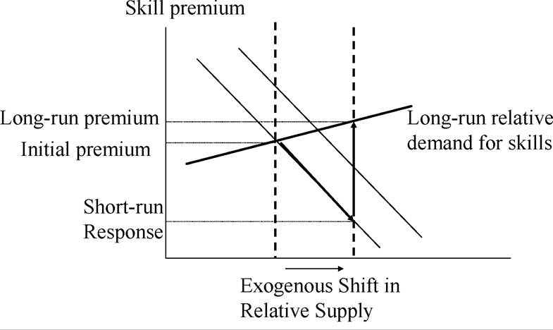
(2) Acceleration in the increase in the number of skilled workers over the past 25 years, shown in Figure 15.1, should induce an acceleration in skill-biased technological change. We will also discuss below how this class of models might account for the dynamics of factor prices in the face of endogenously changing technologies.

(3) Can the framework also explain the prevalence of skill-replacing/labor-biased tech­nological change in the late 18th and 19th centuries? While we know less about both changes in relative supplies and technological developments during these historical periods, available evidence suggests that there were large increases in the number of unskilled workers available to be employed in the factories during this time periods. Bairoch (1988, p. 245), for example, describes this rapid expansion of the supply of unskilled labor as follows:

“... between 1740 and 1840 the population of England... went up from 6 million to 15.7 million.... while the agricultural labor force represented 60-70% of the total work force in 1740, by 1840 it represented only 22%.”

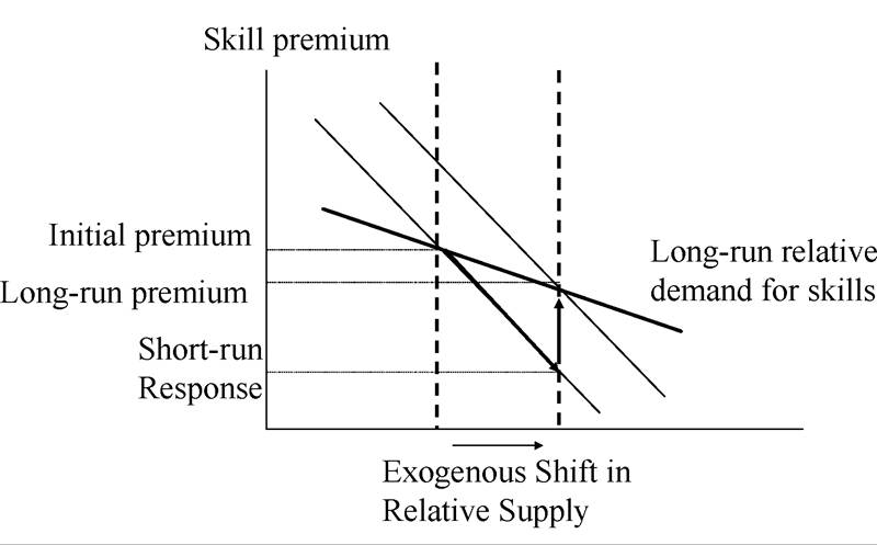
Habakkuk’s well-known account of 19th-century technological development (pp. 136-137) also emphasizes the increase in the supply of unskilled labor in English cities, and attributes it to five sources. First, “technical changes in agriculture increased the supply of labor available to industry” (p. 137). Second, “population was increasing very rapidly” (p. 136). Third, labor reserves of rural industry came to the cities. Fourth, “there was a large influx of labor from Ireland” (p. 137). Finally, enclosures released substantial labor from agriculture.^{[30] [31] According to our model of directed technological change, this increase in the relative supply of unskilled labor should have encouraged unskill-biased technical change, and this is consistent with the patterns discussed above.}

In addition to accounting for the recent skill-biased technological developments and for the historical technologies that appear to have been biased towards unskilled workers, this framework also gives a potential interpretation for the dynamics of the college premium during the 1970s and 1980s. It is reasonable to presume that the equilibrium skill bias of technologies, Nh/Nl, is a sluggish variable determined by the slow buildup and development of new technologies (as the analysis of transitional dynamics in Proposition 15.2 shows). In this case, a rapid increase in the supply of skills would first reduce the skill premium as the economy would be moving along a constant technology (constant Nh/Nl) curve as shown in Figure 15.4. After a while technology would start adjusting, and the economy would move back to the upward sloping relative demand curve, with a relatively sharp increase in the college premium. This approach can therefore explain both the decline in the college premium during the 1970s and its subsequent large surge, and relates both of these phenomena to the large increase in the supply of skilled workers.

If on the other hand we have σ < 2, the long-run relative demand curve will be downward sloping, though again it will be shallower than the short-run relative demand curve. Following the increase in the relative supply of skills there will again be an initial decline in the college premium, and as technology starts adjusting the skill premium will increase. But it will end

Figure 15.4. Dynamics of the skill premium in response to an exogenous increase in the relative supply of skills, with an upward-sloping endogenous- technology relative demand curve.

up below its initial level. To explain the larger increase in the college premium in the 1980s, in this case we would need some exogenous skill-biased technical change. Figure 15.5 draws this case.

Consequently, a model of directed technological change can shed light both on the secular skill bias of technology and on the relatively short-run changes in technology-induced factor prices. We will study other implications of these results below. However, before doing this, a couple of further issues need to be discussed. First, Proposition 15.4 shows that upward-sloping relative demand curves arise only when σ > 2. In the context of substitution between skilled and unskilled workers, an elasticity of substitution much higher than 2 is unlikely. Most estimates put the elasticity of substitution between 1.4 and 2. One would like to understand whether σ > 2 is a feature of the specific model discussed here and how different assumptions about the technology of production or the innovation possibilities frontier affect this result. This issue will be discussed in Section 15.4. Second, we would like to understand the relationship between the market size effect and the scale effects, in particular, whether the results on induced technological change are an artifact of the scale effect (which many economists do not view as an attractive feature of endogenous technological change models). Section 15.5 shows that this is not the case and exactly the same results apply 583

Figure 15.5. Dynamics of the skill premium in response to an increase in the relative supply of skills, with a downward-sloping endogenous-technology relative demand curve.

when scale effects are removed. Third, we would like to apply these ideas to investigate whether there are reasons for technological change to be endogenously labor-augmenting in the neoclassical growth model. This will be investigated in Section 15.6. Finally, it is also useful to contrast equilibrium allocation to the Pareto optimal allocation. We will start with this latter comparison in the next subsection.

15.3.4. Pareto Optimal Allocations. The analysis of Pareto optimal allocation is very similar to the analysis of optimal growth in Chapter 13. For this reason, we will present only a sketch of the argument. As in that analysis, it is straightforward to see that the social planner would not charge a markup on machines, thus we have

Combining these with the production function and some algebra establish that net output, which can be used for consumption or research, is equal to (see Exercise 15.6):

In view of this, the current-value Hamiltonian for the social planner can be written as

subject to

The necessary conditions for this problem give the following characterization of the Pareto optimal allocation in this economy.

Proposition 15.5. The stationary solution of the Pareto optimal allocation involves relative technologies given by (15.27) as in the decentralized equilibrium. The stationary growth rate is higher than the equilibrium growth rate and is given by

where g* is the BGP growth rate given in (15.29).

Proof. See Exercise 15.7. ?

15.4.