Directed Technological Change with Knowledge Spillovers

I now consider the directed technological change model of the previous section with knowl­edge spillovers. This exercise has three purposes. First, it will show how the main results on the direction of technological change can be generalized to a model using the other common specification of the innovation possibilities frontier.

The lab equipment specification of the innovation possibilities frontier is special in one respect: it does not allow for state dependence. State dependence refers to the phenomenon in which the path of past innovations affects the relative costs of different types of innovations. The lab equipment specification implied that R&D spending always leads to the same increase in the number of L-augmenting and H-augmenting machines. We will now introduce a specification with knowledge spillovers, which allows for state dependence. Recall that, as discussed in Section 13.2 in Chapter 13, when there are scarce factors used for R&D, then growth cannot be sustained by continuously increasing the amount of these factors allocated to R&D. Therefore, in order to achieve sustained growth, these factors need to become more and more productive over time, because of spillovers from past research. Here for simplicity, let us assume that R&D is carried out by scientists and that there is a constant supply of scientists equal to S (Exercise 15.18 shows that the results are identical when workers can be employed in the R&D sector). With only one sector, the analysis in Section 13.2 in Chapter 13 indicates that sustained endogenous growth requires N/N to be proportional to S. With two sectors, instead, there is a variety of specifications with different degrees of 585

state dependence, because productivity in each sector can depend on the state of knowledge in both sectors.

(15.32)

where δ ≤ 1, and Sl (t) is the number of scientists working to produce L-augmenting ma­chines, while Sh (t) denotes the number of scientists working on H-augmenting machines. Clearly, market clearing for scientists requires that

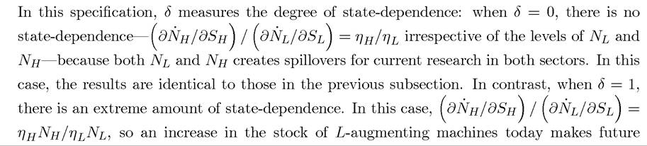
labor-complementary innovations cheaper, but has no effect on the cost of H-augmenting innovations. This discussion clarifies the role of the parameter δ and the meaning of state dependence. In some sense, state dependence adds another layer of “increasing returns,” this time not for the entire economy, but for specific technology lines. In particular, a significant amount of state dependence implies that when Nh is high relative to Nl, it becomes more profitable to undertake more Nh-type innovations.

With this formulation of the innovation possibilities frontier, the free entry conditions become (see Exercise 15.8):

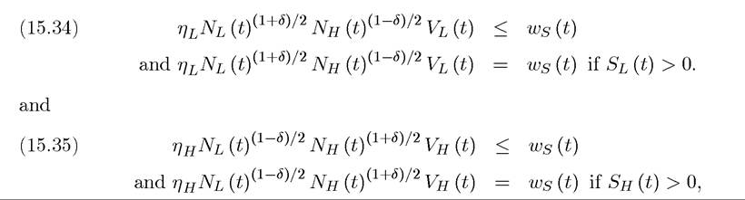
where ws (t) denotes the wage of a scientist at time t. When both of these free entry conditions hold, BGP technology market clearing implies

where δ captures the importance of state-dependence in the technology market clearing con­dition, and profits are not conditioned on time, since they refer to the BGP values, which are constant as in the previous section (recall (15.15)). When δ = 0, this condition is identical to (15.26) in the previous section. Therefore, as claimed above, all of the results concerning 586

the direction of technological change would be identical to those from the lab equipment specification.

This is no longer true when δ > 0. To characterize the results in this case, let us combine condition (15.36) with equations (15.15) and (15.18), we obtain the equilibrium relative technology as (see Exercise 15.9):

between the relative factor supplies and relative physical productivities now depends on δ. This is intuitive: as long as δ > 0, an increase in Nh reduces the relative costs of H- augmenting innovations, so for technology market equilibrium to be restored, ∏l needs to fall relative to π∣∕. Substituting (15.37) into the expression for relative factor prices for given technologies, which is still (15.19), yields the following long-run (endogenous-technology) relationship between relative factor prices and relative factor supplies:

It can be verified that when δ = 0,so that there is no state-dependence in R&D, both of the previous expressions are identical to their counterparts in the previous section.

The growth rate of this economy is determined by the number of scientists. In BGP, both Combining this equation with (15.33) and (15.37), we obtain the following BGP condition for the allocation of researchers between the two different types of technologies,

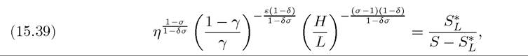
and the BGP growth rate (15.40) below. Notice that given H/L, the BGP researcher alloca­tions,andare uniquely determined. We summarize these results with the following proposition:

PropoSITION 15.6.

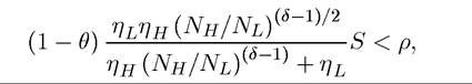
where Nh/Nl is given by (15.37). Then there exists a unique BGP equilibrium in which the relative technologies are given by (15.37), and consumption and output grow at the rate

587

Proof. See Exercise 15.10. ?

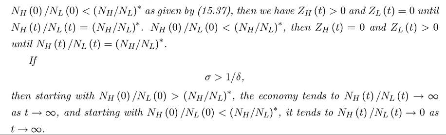
In contrast to the model with the lab equipments technology, transitional dynamics do not always take the economy to the BGP equilibrium, however. This is because of the additional increasing returns to scale mentioned above. With a high degree of state dependence, when Nh (0) is very high relative to Nl (0), it may no longer be profitable for firms to undertake further R&D directed at labor-augmenting (L-augmenting) technologies. Whether this is so or not depends on a comparison of the degree of state dependence, δ, and the elasticity of substitution, σ. The latter matters because it regulates how prices change as there is an abundance of one type of technology relative to another, and thus determines the strength of the price effect on the direction of technological change. The next proposition analyzes the transitional dynamics in this case.

PROPOSITION 15.7. Consider the directed technological change model with knowledge spillovers and state dependence in the innovation possibilities frontier. Suppose that

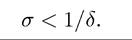
Then, starting with any N∣∣ (0) > 0 and Nl (0) > 0, there exists a unique equilibrium path. If

Proof. See Exercise 15.12. ?

Of greater interest for our focus are the results on the direction of technological change.

PROPOSITION 15.8. Consider the directed technological change model with knowledge spil lovers and state dependence in the innovation possibilities frontier. Then there is al­ways weak equilibrium (relative) bias in the sense that an increase in H/L always induces relatively H-biased technological change.

Proof. See Exercise 15.13. ?

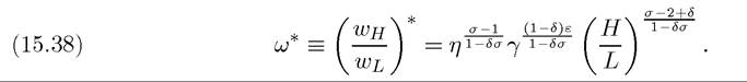
While the results regarding weak bias have not changed, inspection of (15.38) shows that it is now easier to obtain strong equilibrium (relative) bias.

PROPOSITION 15.9. Consider the directed technological change model with knowledge spillovers and state dependence in the innovation possibilities frontier. Then if there is strong equilibrium (relative) bias in the sense that an increase in H/L raises the relative marginal product and the relative wage of the H factor compared to the L factor.

Intuitively, the additional increasing returns to scale coming from state dependence makes strong bias easier to obtain, because the induced technology effect is stronger. When a particular factor, say H, becomes more abundant, this encourages an increase in N∏ relative to Nl (in the case where σ > 1). However, from state dependence, this makes further increases in Nh more profitable, thus has a larger effect on Nh/Nr. Since with σ > 1 greater values of Nh/Nl tend to increase the relative price of factor H compared to L, this tends to make the strong bias result easier to obtain.

Returning to our discussion of the implications of the strong bias results for the behavior of the skill premium in the U.S. market, Proposition 15.9 implies that values of the elasticity of substitution between skilled and unskilled labor significantly less than 2 may be sufficient to generate strong equilibrium bias. How much lower than 2 the elasticity of substitution can be depends on the parameter δ. Unfortunately, this parameter is not easy to measure in practice, even though existing evidence suggests that there is some amount of state dependence in the R&D technologies. For example, this is confirmed by the empirical finding that most patents developed in a particular industry build upon and cite previous patents in the same industry.

15.5.