Brief Review of Dynamic Programming

Using abstract but simple notation, the canonical dynamic optimization program in dis­crete time can be written as

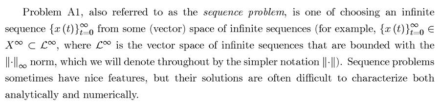
Problem A1 :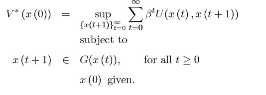

Again the added generality in this case is not particularly useful for most of the problems we are interested in, and the discounted objective function ensures time-consistency as discussed in the previous chapter.

Of particular importance for us in this chapter is the function V * (x (0)), which can be thought of as the value function, meaning the value of pursuing the optimal strategy starting with initial state x (0).

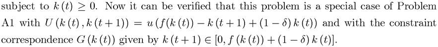
Problem A1 is somewhat abstract. However, it has the advantage of being tractable and general enough to nest many interesting economic applications. The next example shows how our canonical optimal growth problem can be put into this language.

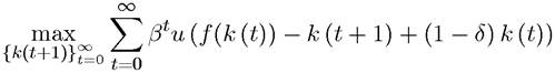
EXAMPLE 6.1. Recall the optimal growth problem from the previous chapter:

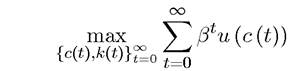
subject to

k (t + 1) — f (k (t)) — c (t) + (1 — δ) k (t),

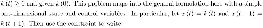
c (t) — f (k (t)) — k (t + 1) + (1 — δ) k (t),

and substitute this into the objective function to obtain:

The basic idea of dynamic programming is to turn the sequence problem into a functional equation. That is, it is to transform the problem into one of finding a function rather than a 217

sequence.

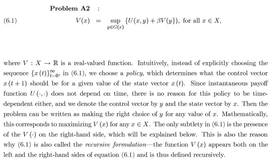
The functional equation in Problem A2 is also called the Bellman equation, after Richard Bellman, who was the first to introduce the dynamic programming formulation, though this formulation was anticipated by the economist Lloyd Shapley in his study of stochastic games.

At first sight, the recursive formulation might appear not as a great advance over the sequence formulation. After all, functions might be trickier to work with than sequences. Nevertheless, it turns out that the functional equation of dynamic programming is easy to work with in many instances. In applied mathematics and engineering, it is favored because it is computationally convenient. In economics, perhaps the major advantage of the recursive formulation is that it often gives better economic insights, similar to the logic of comparing today to tomorrow. In particular, U (x,y^) is the“ return for today” and is the continuation return from tomorrow onwards, equivalent to the “return for tomorrow”. Consequently, in many applications we can use our intuitions from two-period maximization or economic problems. Finally, in some special but important cases, the solution to Problem A2 is simpler to characterize analytically than the corresponding solution of the sequence problem, Problem A1.

In fact, the form of Problem A2 suggests itself naturally from the formulation Problem A1. Suppose Problem A1 has a maximum starting at x (0) attained by the optimal sequence 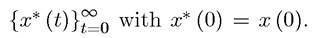Then under some relatively weak technical conditions, we

have that

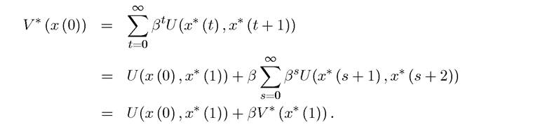
This equation encapsulates the basic idea of dynamic programming: the Principle of Opti­mality, and it is stated more formally in Theorem 6.2.

Essentially, an optimal plan can be broken into two parts, what is optimal to do today, and the optimal continuation path. Dynamic programming exploits this principle and provides us with a set of powerful tools to analyze optimization in discrete-time infinite-horizon problems.

As noted above, the particular advantage of this formulation is that the solution can be represented by a time invariant policy function (or policy mapping), 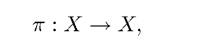determining which value of x (t + 1) to choose for a given value of the state variable x (t). In general, however, there will be two complications: first, a control reaching the optimal value may not exist, which was the reason why we originally used the notation sup; second, we may not have a policy function, but a policy correspondence,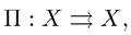because there may

be more than one maximizer for a given state variable. Let us ignore these complications for now and present a heuristic exposition. These issues will be dealt with below.

Once the value function V is determined, the policy function is given straightforwardly. In particular, by definition it must be the case that if optimal policy is given by a policy function π (x), then 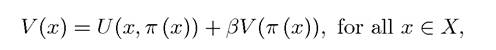which is one way of determining the policy function. This equation simply follows from the fact thatis the optimal policy, so whenthe right-hand side of (6.1) reaches

the maximal value V (x).

The usefulness of the recursive formulation in Problem A2 comes from the fact that there are some powerful tools which not only establish existence of the solution, but also some of its properties. These tools are not only employed in establishing the existence of a solution to Problem A2, but they are also useful in a range of problems in economic growth, macroeconomics and other areas of economic dynamics.

The next section states a number of results about the relationship between the solution to the sequence problem, Problem A1, and the recursive formulation, Problem A2. These 219

results will first be stated informally, without going into the technical details. Section 6.3 will then present these results in greater formality and provide their proofs.

6.2.