Dynamic Programming Theorems

Let us start with a number of assumptions on Problem A1. Since these assumptions are only relevant for this section, we number them separately from the main assumptions used throughout the book.

and that any solution to (6.2) will also be a solution to Problem A1, in the sense that it will attain its supremum. In other words, we are interested in in establishing equivalence results between the solutions to Problem A1 and Problem A2.

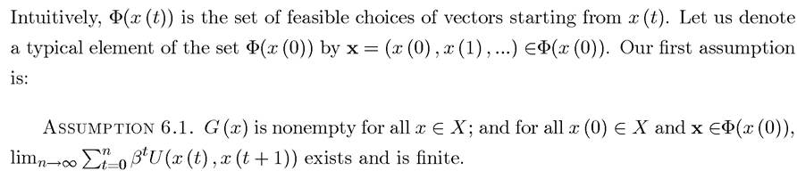
To prepare for these results, let us define the set of feasible sequences or plans starting with an initial value x (t) as:

This assumption is stronger than what is necessary to establish the results that will follow. In particular, for much of the theory of dynamic programming, it is sufficient that the limit in Assumption 6.1 exists. However, in economic applications, we are not interested in optimization problems where households or firms achieve infinite value. This is for two obvious reasons. First, when some agents can achieve infinite value, the mathematical problems are typically not well defined. Second, the essence of economics, tradeoffs in the face of scarcity, would be absent in these cases. In cases, where households can achieve infinite value, economic analysis is still possible, by using methods sometimes called “overtaking criteria,” whereby different sequences that give infinite utility are compared by looking at whether one of them gives higher utility than the other one at each date after some finite threshold.

This assumption is also natural. We need to impose that G (x) is compact-valued, since optimization problems with choices from non-compact sets are not well behaved (see Ap­pendix Chapter A). In addition, the assumption that U is continuous leads to little loss of generality for most economic applications. In all the models we will encounter in this book, U will be continuous. The most restrictive assumption here is that the state variable lies in a compact set, i.e., that X is compact. The most important results in this chapter can be generalized to the case in which X is not compact, though this requires additional notation and somewhat more difficult analysis. The case in which X is not compact is important in the analysis of economic growth, since most interesting models of growth will involve the state variable, e.g., the capital stock, growing steadily. In many cases, with a convenient normalization, the mathematical problem can be turned in to one in which the state vari­able lies in a compact set. One class of important problems that cannot be treated without allowing for non-compact X are those with endogenous growth. However, since the methods developed in the next chapter do not require this type of compactness assumption and since I will often use continuous-time methods to study endogenous growth models, I simplify the discussion here by assuming that X is compact.

Note also that since X is compact, G (x) is continuous and compact-valued, X_g is also compact. Since a continuous function from a compact domain is also bounded, Assumption 6.2 also implies that U is bounded, which will be important for some of the results below.

Assumptions 6.1 and 6.2 together ensure that in both Problems A1 and A2, the supremum (the maximal value) is attained for some feasible plan x. We state all the relevant theorems incorporating this fact.

To obtain sharper results, we will also impose:

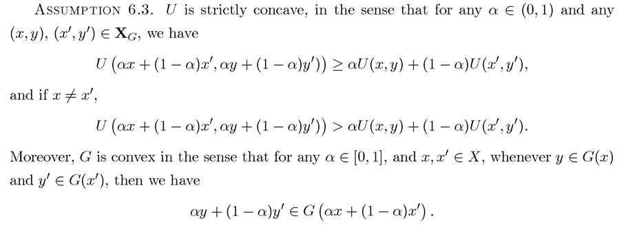
This assumption imposes conditions similar to those used in many economic applications: the constraint set is assumed to be convex and the objective function is concave or strictly concave.

Our next assumption puts some more structure on the objective function, in particular it ensures that the objective function is increasing in the state variables (its first K arguments), and that greater levels of the state variables are also attractive from the viewpoint of relaxing the constraints; i.e., a greater x means more choice.

The final assumption we will impose is that of differentiability and is also common in most economic models. This assumption will enable us to work with first-order necessary conditions.

Assumption 6.5. U is continuously differentiable on the interior of its domain Xg.

Given these assumptions, the following sequence of results can be established. The proofs for these results are provided in Section 6.4.

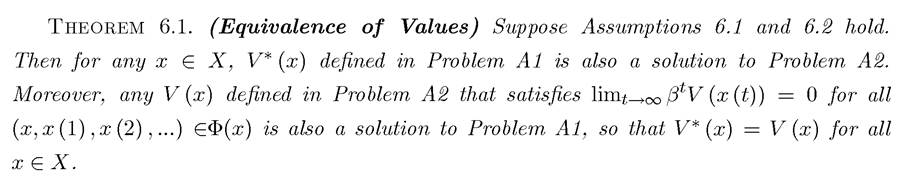
Therefore, both the sequence problem and the recursive formulation achieve the same value. While important, this theorem is not of direct relevance in most economic applications, since we do not care about the value but we care about the optimal plans (actions). This is dealt with in the next theorem.

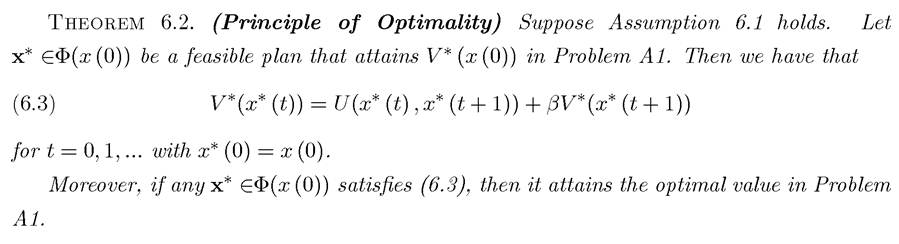
This theorem is the major conceptual result in the theory of dynamic programming. It states that the returns from an optimal plan (sequence)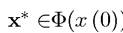) can be broken into two

parts; the current return,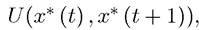and the continuation return

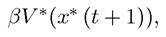
where the continuation return is identically given by the discounted value of a problem

222

starting from the state vector from tomorrow onwards, x* (t + 1). In view of the fact that V * in Problem A1 and V in Problem A2 are identical from Theorem 6.1, (6.3) also implies

Notice also that the second part of Theorem 6.2 is equally important. It states that if any feasible plan x* starting with x (0), that is,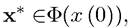satisfies (6.3), then x* attains

Therefore, this theorem states that we can go from the solution of the recursive problem to the solution of the original problem and vice versa.

The next results summarize certain important features of the value function V in Problem A2. These results will be useful in characterizing qualitative features of optimal plans in dynamic optimization problems without explicitly finding the solutions.

Theorem 6.3. (Existence of Solutions) Suppose that Assumptions 6.1 and 6.2 hold. Then there exists a unique continuous and bounded functionthat satisfies (6.1).

Moreover, an optimal planexists for any

This theorem establishes two major results. The first is the uniqueness of the value function (and hence of the Bellman equation) in dynamic programming problems. Combined with Theorem 6.1, this result naturally implies that an optimal solution that achieves the supremum V^* in Problem A1 and also that like V, V^* is continuous and bounded. The optimal solution to Problem A1 or A2 may not be unique, however, even though the value function is unique. This may be the case when two alternative feasible sequences achieve the same maximal value. As in static optimization problems, non-uniqueness of solutions is a consequence of lack of strict concavity of the objective function. When the conditions are strengthened by including Assumption 6.3, uniqueness of the optimum will plan is guaranteed. To obtain this result, we first prove:

Theorem 6.4. (Concavity of the Value Function) Suppose that Assumptions 6.1, 6.2 and 6.3 hold. Then the unique V : X → R that satisfies (6.1) is strictly concave.

Combining the previous two theorems we have:

COROLLARY 6.1. Suppose that Assumptions 6.1, 6.2 and 6.3 hold.

The important result in this corollary is that the “policy function” π is indeed a function, not a correspondence. This is a consequence of the fact that x^* is uniquely determined. This result also implies that the policy mapping π is continuous in the state vector. Moreover, if 223

there exists a vector of parameters z continuously affecting either the constraint correspon­dence Φ or the instantaneous payoff function U, then the same argument establishes that π is also continuous in this vector of parameters. This feature will enable qualitative analysis of dynamic macroeconomic models under a variety of circumstances.

Our next result shows that under Assumption 6.4, we can also establish that the value function V is strictly increasing.

Theorem 6.5. (Monotonicity of the Value Function) Suppose that Assumptions 6.1, 6.2 and 6.4 hold and let V :be the unique solution to (6.1). Then V is strictly

increasing in all of its arguments.

Finally, our purpose in developing the recursive formulation is to use it to characterize the solution to dynamic optimization problems. As with static optimization problems, this is often made easier by using differential calculus. The difficulty in using differential calculus with (6.1) is that the right-hand side of this expression includes the value function V, which is endogenously determined. We can only use differential calculus when we know from more primitive arguments that this value function is indeed differentiable. The next theorem ensures that this is the case and also provides an expression for the derivative of the value function, which corresponds to a version of the familiar Envelope Theorem. Recall that IntX denotes the interior of the set X, D_x f denotes the gradient of the function f with respect to the vector x, and Df denotes the gradient of the function f with respect to all of its arguments (see Appendix Chapter A).

Theorem 6.6. (Differentiability of the Value Function) Suppose that Assumptions 6.1, 6.2, 6.3 and 6.5 hold. Let π be the policy function defined above and assume that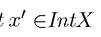 and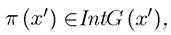then V (x) is continuously differentiable at x', with derivative given by

(6.4)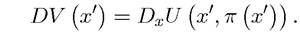

These results will enable us to use dynamic programming techniques in a wide variety of dynamic optimization problems. Before doing so, we discuss how these results are proved. The next section introduces a number of mathematical tools from basic functional analysis necessary for proving some of these theorems and Section 6.4 provides the proofs of all the results stated in this section.

6.3.