The Contraction Mapping Theorem and Applications*
In this section, I present a number of mathematical results that are necessary for making progress with the dynamic programming formulation. In this sense, the current section is a “digression” from the main story line.
Therefore, this section and the next can be skipped without interfering with the study of the rest of the book. Nevertheless, the material in this 224and the next section are useful for a good understanding of foundations of dynamic programming and should enable the reader to achieve a better understanding of these methods. The reader may also wish to consult Appendix Chapter A before reading this section.
Recall from Appendix Chapter A that (S, d) is a metric space, if S is a space and d is a metric de fined over this space with the usual properties. The metric is referred to as “d” since it loosely corresponds to the “distance” between two elements of S. A metric space is more general than a finite dimensional Euclidean space such as a subset of . But as with the Euclidean space, we are most interested in defining “functions” from the metric space into itself. We will refer to these functions as operators or mappings to distinguish them from real-valued functions. Such operators are often denoted by the letter T and standard notation often involves writing Tz for the image of a point
 under T (rather than the more intuitive and familiar T (z)), and using the notation T (Z) when the operator T is applied to a subset Z of S. We will use this standard notation here.
Definition 6.1. Let (S,d) be a metric space and be an operator mapping S
into itself.
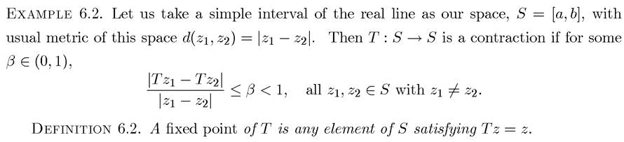
T is a contraction mapping (with modulus

In other words, a contraction mapping brings elements of the space S “closer” to each other.
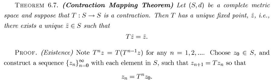
Recall also that a metric space (S, d) is complete if every Cauchy sequence (whose elements are getting closer) in S converges to an element in S (see Appendix Chapter A). Despite its simplicity, the following theorem is one of the most powerful results in functional analysis.
225
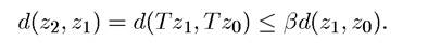
Since T is a contraction, we have that
Repeating this argument
(6.5) 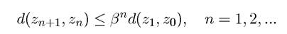
Hence, for any m > n,
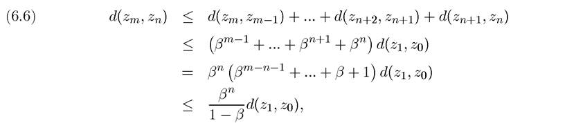
where the first inequality uses the triangle inequality (which is true for any metric d, see Appendix Chapter A). The second inequality uses (6.5). The last inequality uses the fact

The string of inequalities in (6.6) imply that l will be
approaching each other, so that is a Cauchy sequence. Since S is complete, every Cauchy sequence in S has an limit point in S, therefore:
The next step is to show that z is a fixed point.
Note that for any zo ∈ S and any n ∈ N, we have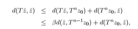
where the first relationship again uses the triangle inequality, and the second inequality utilizes the fact that T is a contraction. Since both of the terms on the right tend to zero as n → ∞, which implies that
 and therefore
 establishing that
z is a fixed point.
(Uniqueness) Suppose, to obtain a contradiction, that there exist such that
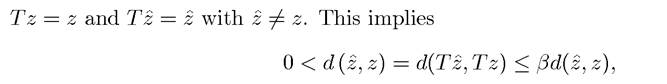
which delivers a contradiction in view of the fact that and establishes uniqueness. ?
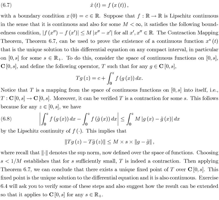
The Contraction Mapping Theorem can be used to prove many well-known results. The next example and Exercise 6.4 show how it can be used to prove existence of unique solutions to differential equations. Exercise 6.5 shows how it can be used to prove the Implicit Function Theorem (Theorem A.23 in Appendix Chapter A).
Example 6.3. Consider the following one-dimensional differential equation
The main use of the Contraction Mapping Theorem for us is that it can be applied to any metric space, so in particular to the space of functions. Applying it to equation (6.1) will establish the existence of a unique value function V in Problem A2, greatly facilitating the analysis of such dynamic models. Naturally, for this we have to prove that the recursion in (6.1) defines a contraction mapping.
We will see below that this is often straightforward.Before doing this, let us consider another useful result. Recall that if (S, d) is a complete metric space and S0 is a closed subset of S, then (S0,d) is also a complete metric space.
Theorem 6.8. (Applications of Contraction Mappings) Let (S,d) be a complete metric space,
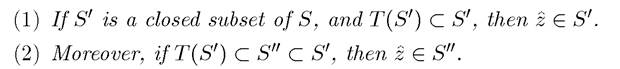
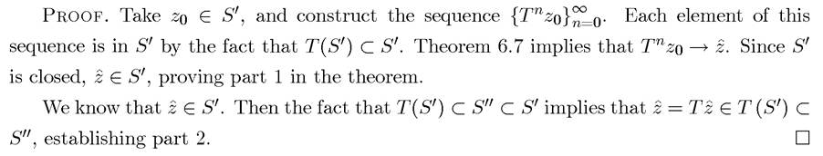
The second part of this theorem is very important to prove results such as strict concavity or that a function is strictly increasing. This is because the set of strictly concave functions or the set of the strictly increasing functions are not closed (and complete). Therefore, we cannot apply the Contraction Mapping Theorem to these spaces of functions. The second part of this theorem enables us to circumvent this problem.
The previous two theorems show that the contraction mapping property is both simple and powerful. We will see how powerful it is as we apply to obtain several important results below. Nevertheless, beyond some simple cases, such as Example 6.2, it is difficult to check whether an operator is indeed a contraction. This may seem particularly difficult in the case of spaces whose elements correspond to functions, which are those that are relevant in the context of dynamic programming. The next theorem provides us with sufficient conditions for an operator to be a contraction that are typically straightforward to check. For this theorem, let us use the following notation: for a real valued function f (∙) and some constant c ∈ R we define (f + c)(x) ? f (x) + c. Then:
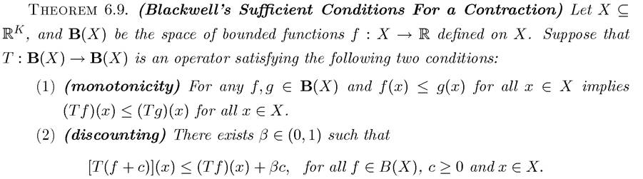
Then, T is a contraction with modulus β.
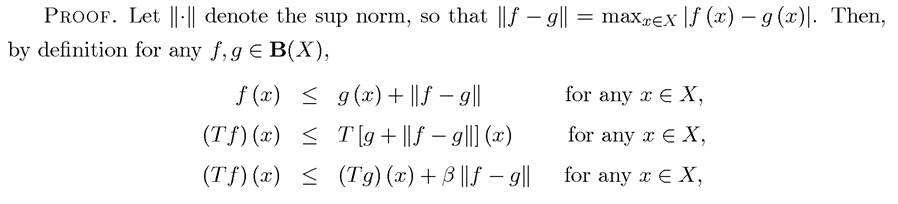
where the second line applies the operator T on both sides and uses monotonicity, and the third line uses discounting (together with the fact that is simply a number). By the 228
converse argument,
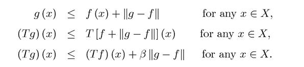
Combining the last two inequalities implies

proving that T is a contraction. ?
We will see that Blackwell’s sufficient conditions are straightforward to check in many economic applications, including the models of optimal or equilibrium growth.
6.4.