Proofs of the Main Dynamic Programming Theorems*
We now prove Theorems 6.1-6.6. We start with a straightforward lemma, which will be useful in these proofs. For a feasible infinite sequence starting
at x (0), let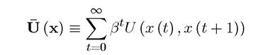
be the value of choosing this potentially non-optimal infinite feasible sequence.
In view of Assumption 6.1, U (x) exists and is finite. The next lemma shows that U (x) can be separated into two parts, the current return and the continuation return.LEMMA 6.1. Suppose that Assumption 6.1 holds. Then for any x (0) ∈ X and any x ∈Φ(x (0)), we have that
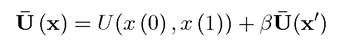
where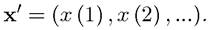
Proof. Since under Assumption 6.1 U (x) exists and is finite, we have
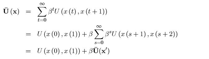
as defined in the lemma. ?
We start with the proof of Theorem 6.1. Before providing this proof, it is useful to be more explicit about what it means for V and V * to be solutions to Problems A1 and A2. Let 229
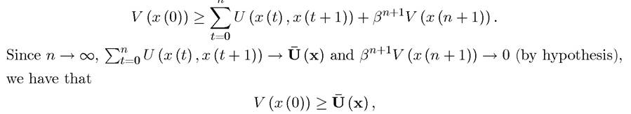
us start with Problem A1. Using the notation introduced in this section, we can write that for any x (0) ∈ X,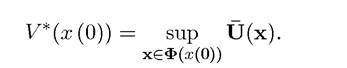
In view of Assumption 6.1, which ensures that all values are bounded, this immediately implies
since no other feasible sequence of choices can give higher value than the supremum, V * (x (0)). However, if some function V satisfies condition (6.9), so will αV for a > 1.
Therefore, this condition is not sufficient. In addition, we also require that
The conditions for V (∙) to be a solution to Problem A2 are similar. For any x (0) ∈ X,  and
and

We now have:
Proof of Theorem 6.1. If β = 0, Problems A1 and A2 are identical, thus the result follows immediately. Suppose that β > 0 and take an arbitrary x (0) ∈ X and some x (1) ∈ G (x (0)). The objective function in Problem A1 is continuous in the product topology in view of Assumptions 6.1 and 6.2 (see Theorem A.11 in Appendix Chapter A). Moreover, the constraint set Φ(x (0)) is a closed subset of X∞ (infinite product of X). From Assumption 6.1, X is compact. By Tychonoff's Theorem, Theorem A.12, X∞ is compact in the product topology. A closed subset of a compact set is compact (Fact A.2 in Appendix Chapter A), which implies that Φ(x (0)) is compact. Thus we can apply Weierstrass' Theorem, Theorem A.9, to Problem A1, to conclude that there exists x ∈Φ(x (0)) attaining V * (x (0)). Moreover, the constraint set is a continuous correspondence (again in the product topology), so Berge's Maximum Theorem, Theorem A.13, implies that V * (x(0)) is continuous. Since x (0) ∈ X and X is compact, this implies that V * (x (0)) is bounded (Corollary A.1 in Appendix Chapter A). A similar reasoning implies that there exists x0∈Φ(x (1)) attaining V* (x (1)). Next, since (x (0), x0) ∈Φ(x (0)) and V * (x (0)) is the supremum in Problem A1 starting with x (0), Lemma 6.1 implies
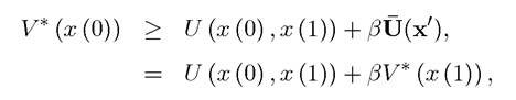
thus verifying (6.11).
Next, take an arbitrary ε > 0.
By (6.10), there exists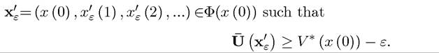
 is the supremum in Problem A1 starting with x'ε (1), Lemma 6.1 implies
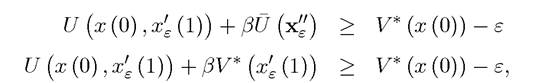
The last inequality verifies (6.12) since for any ε > 0. This proves that any
solution to Problem A1 satisfies (6.11) and (6.12), and is thus a solution to Problem A2.
To establish the reverse, note that (6.11) implies that for any x (1) ∈ G (x (0)),

Now substituting recursively for V (x (1)), V (x (2)), etc., and defining x = (x (0),x (1),...), we have
for any x ∈Φ(x (0)), thus verifying (6.9).
Next, let ε > 0 be a positive scalar. From (6.12), we have that for any there exists xε (1) ∈G (x (0)) such that

id="Picutre 571" class="lazyload" data-src="/files/uch_group77/uch_pgroup317/uch_uch7364/image/image571.jpg">Again substituting recursively for V (xε (1)), V (xε (2)),..., we obtain
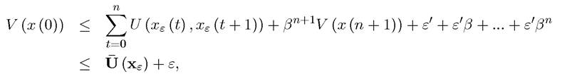
where the last step follows using the definition of ε (in particular that ) and
) and
because as This establishes that V (0) satisfies
(6.10), and completes the proof.
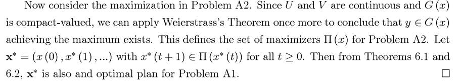
?In economic problems, we are often interested not in the maximal value of the program but in the optimal plans that achieve this maximal value. Recall that the question of whether the optimal path resulting from Problems A1 and A2 are equivalent was addressed by Theorem
6.2. We now provide a proof of this theorem.
Proof of Theorem 6.2. By hypothesis is a solution
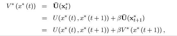
to Problem A1, i.e., it attains the supremum, V * (x (0)) starting from x (0). Let x* ? (x* (t),x* (t + 1),...).
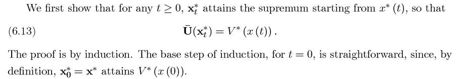
Next suppose that the statement is true for t, so that (6.13) is true for t, and we will establish it for t + 1. Equation (6.13) implies that
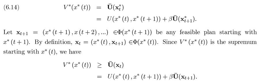
Combining this inequality with (6.14), we obtain


Equation (6.13) then implies that
establishing (6.3) and thus completing the proof of the first part of the theorem.
Now suppose that (6.3) holds for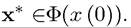 Then substituting repeatedly for x*, we
obtain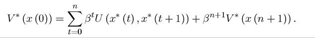
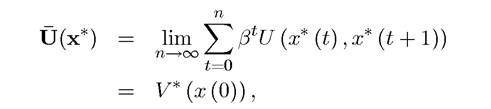
In view of the fact that V * (∙) is bounded, we have that
232
thus x* attains the optimal value in Problem A1, completing the proof of the second part of the theorem. ?
We have therefore established that under Assumptions 6.1 and 6.2, we can freely interchange Problems A1 and A2.
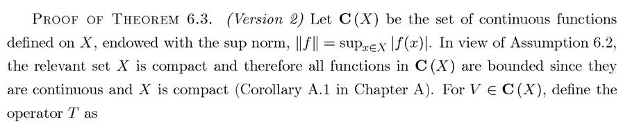
Our next task is to prove that a policy achieving the optimal path exists for both problems. We will provide two alternative proofs for this to show how this conclusion can be reached either by looking at Problem A1 or at Problem A2, and then exploiting their equivalence. The first proof is more abstract and works directly on the sequence problem, Problem A1.Proof of Theorem 6.3. (Version 1) Consider Problem A1. The argument at the beginning of the proof of Theorem 6.1 again enables us to apply Weierstrass’s Theorem, Theorem A.9 to conclude that an optimal path ?
?
(6.15)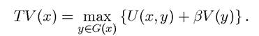
A fixed point of this operator, V = TV, will be a solution to Problem A2. We first prove that such a fixed point (solution) exists. The maximization problem on the right-hand side of (6.15) is one of maximizing a continuous function over a compact set, and by Weierstrass’s Theorem, Theorem A.9, it has a solution. Consequently, T is well-defined. Moreover, because G (x^) is a nonempty and continuous correspondence by Assumption 6.1 and U (x,y^) and V (y) are continuous by hypothesis, Berge’s Maximum Theorem, Theorem A.13, implies that

Next, it is also straightforward to verify that T satisfies Blackwell’s sufficient conditions for a contraction in Theorem 6.9 (see Exercise 6.6). Therefore, applying Theorem 6.7, a unique fixed point to (6.15) exists and this is also the unique solution to Problem
A2.
233
These two proofs illustrate how different approaches can be used to reach the same conclusion, once the equivalences in Theorems 6.1 and 6.2 have been established.
An additional result that follows from the second version of the theorem (which can also be derived from version 1, but would require more work), concerns the properties of the correspondence of maximizing values
An immediate application of the Theorem of the Maximum, Theorem A.13 in Appendix Chapter A, implies that Π is a upper hemi-continuous and compact-valued correspondence. This observation will be used in the proof of Corollary 6.1. Before turning to this corollary, we provide a proof of Theorem 6.4, which shows how Theorem 6.8 can be useful in establishing a range of results in dynamic optimization problems.
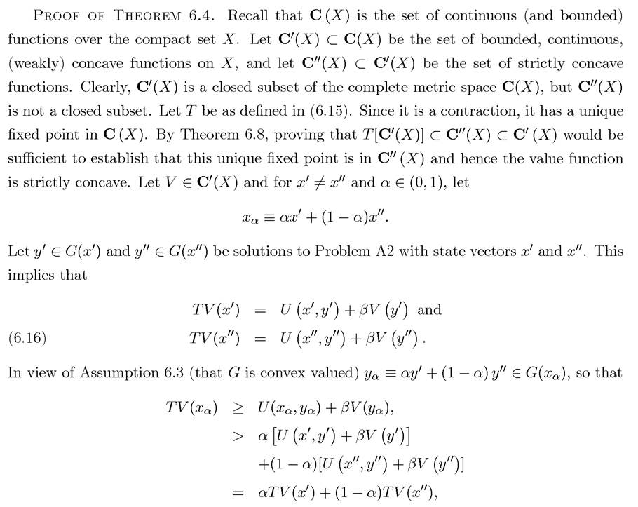
where the first line follows by the fact that yα ∈ G (xα) is not necessarily the maximizer. The second line uses Assumption 6.3 (strict concavity of U), and the third line is simply the definition introduced in (6.16). This argument implies that for any is strictly
234
concave, thus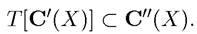 Then Theorem 6.8 implies that the unique fixed point
is in and hence it is strictly concave. ?
proof OF Corollary 6.1. Assumption 6.3 implies that U (x,y) is concave in y, and under this assumption, Theorem 6.4 established that V (y) is strictly concave in y. The sum of a concave function and a strictly concave function is strictly concave, thus the right-hand side of Problem A2 is strictly concave in y. Therefore, combined with the fact that G (x) is convex for each x ∈ X (again Assumption 6.3), there exists a unique maximizer y ∈ G (x) for each x ∈ X. This implies that the policy correspondence Π (x) is single-valued, thus a function, and can thus be expressed as π (x). Since Π (x) is upper hemi-continuous as observed above, so is π(x). Since an upper hemi-continuous function is continuous, the corollary follows. ?
proof OF Theorem 6.6. From Corollary 6.1, Π (x) is single-valued, thus a function that can be represented by π (x). By hypothesis, and from Assumption 6.2
G is continuous. Therefore, there exists a neighborhood N (x (0)) of x (0) such that π(x (0)) ∈
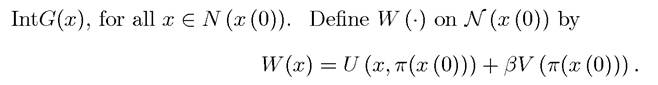
In view of Assumptions 6.3 and 6.5, the fact that is a number (independent of
x), and the fact that U is concave and differentiable, W (∙) is concave and differentiable. Moreover, since π(x (0)) ∈ G(x) for all x ∈ N (x (0)), it follows that

with equality at x (0).
Since V (∙) is concave, -V (∙) is convex, and by a standard result in convex analysis, it possesses subgradients. Moreover, any subgradient p of -V at x (0) must satisfy  where the first inequality uses the definition of a subgradient and the second uses the fact that
 with equality at x (0) as established in (6.17). This implies that every
235
subgradient p of -V is also a subgradient of -W. Since W is differentiable at x (0), its subgradient p must be unique, and another standard result in convex analysis implies that any convex function with a unique subgradient at an interior point x (0) is differentiable at x (0). This establishes that -V (∙), thus V (∙), is differentiable as desired.
The expression for the gradient (6.4) is derived in detail in the next section. ?
6.5.