Fundamentals of Dynamic Programming
In this section, we return to the fundamentals of dynamic programming and show how they can be applied in a range of problems. The main result in this section is Theorem
6.10, which shows how dynamic first-order conditions, the Euler equations, together with the transversality condition are sufficient to characterize solutions to dynamic optimization problems.
This theorem is arguably more useful in practice than the main dynamic programming theorems presented above.6.5.1. Basic Equations. Consider the functional equation corresponding to Problem A2:

Let us assume throughout that Assumptions 6.1-6.5 hold. Then from Theorem 6.4, the maximization problem in (6.18) is strictly concave, and from Theorem 6.6, the maximand is also differentiable. Therefore for any interior solution y ∈IntG (x), the first-order conditions are necessary and sufficient for an optimum. In particular, optimal solutions can be characterized by the following convenient Euler equations:

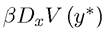
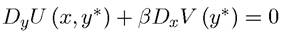
where we use *,s to denote optimal values and once again D denotes gradients (recall that, in the general case, x is a vector not a scalar, thus DxU is a vector of partial derivatives and we denote the vector of partial derivatives of the value function V evaluated at y by DxV (y)).
The set of first-order conditions in equation (6.19) would be sufficient to solve for the optimal policy, y*, if we knew the form of the V (∙) function. Since this function is determined recursively as part of the optimization problem, there is a little more work to do before we obtain the set of equations that can be solved for the optimal policy.
Fortunately, we can use the equivalent of the Envelope Theorem for dynamic programming and differentiate (6.18) with respect to the state vector, x, to obtain:

The reason why this is the equivalent of the Envelope Theorem is that the term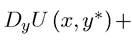
 times the induced change in y in response to the change in x is absent from the expression.
 from (6.19).
 236
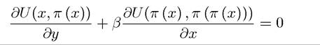
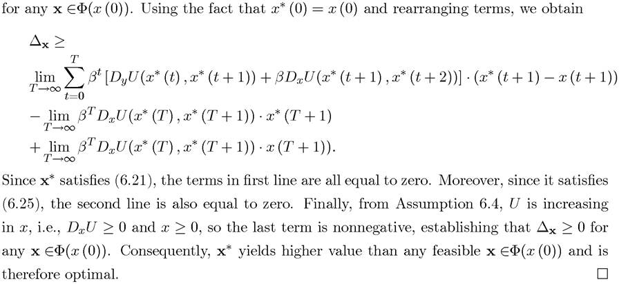
Now using the notation y* = π (x) to denote the optimal policy function (which is singlevalued in view of Assumption 6.3) and the fact that DxV (y) = DxV (π (x)), we can combine these two equations to write

where DxU represents the gradient vector of U with respect to its first K arguments, and Dy U represents its gradient with respect to the second set of K arguments. Notice that (6.21) is a functional equation in the unknown function π (∙) and characterizes the optimal policy function.
These equations become even simpler and more transparent in the case where both x and y are scalars. In this case, (6.19) becomes:
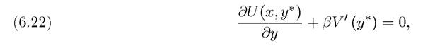
where V0 the notes the derivative of the V function with respect to it single scalar argument.
This equation is very intuitive; it requires the sum of the marginal gain today from increasing y and the discounted marginal gain from increasing y on the value of all future returns to be equal to zero. For instance, as in Example 6.1, we can think of U as decreasing in y and increasing in x; equation (6.22) would then require the current cost of increasing y to be compensated by higher values tomorrow. In the context of growth, this corresponds to current cost of reducing consumption to be compensated by higher consumption tomorrow. As with (6.19), the value of higher consumption in (6.22) is expressed in terms of the derivative of the value function, V0 (y*), which is one of the unknowns. To make more progress, we use the one-dimensional version of (6.20) to find an expression for this derivative:
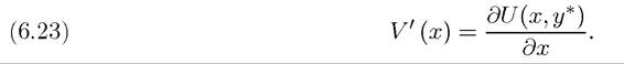
Now in this one-dimensional case, combining (6.23) together with (6.22), we have the following very simple condition:
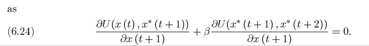
where ∂x denotes the derivative with respect to the first argument and ∂y with respect to the second argument.
Alternatively, we could write the one-dimensional Euler equation with the time arguments
However, this Euler equation is not sufficient for optimality. In addition we need the transver- sality condition. The transversality condition is essential in infinite-dimensional problems, because it makes sure that there are no beneficial simultaneous changes in an infinite number 237
of choice variables. In contrast, in finite-dimensional problems, there is no need for such a condition, since the first-order conditions are sufficient to rule out possible gains when we change many or all of the control variables at the same time. The role that the transversal- ity condition plays in infinite-dimensional optimization problems will become more apparent after we see Theorem 6.10 and after the discussion in the next subsection.
In the general case, the transversality condition takes the form:

where “•” denotes the inner product operator. In the one-dimensional case, we have the simpler transversality condition:
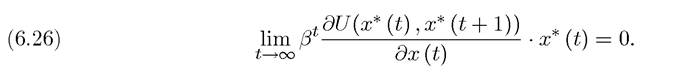
In words, this condition requires that the product of the marginal return from the state variable x times the value of this state variable does not increase asymptotically at a rate faster than
The next theorem shows that the transversality condition together with the transformed Euler equations in (6.21) are sufficient to characterize an optimal solution to Problem A1 and therefore to Problem A2. Exercise 6.11 in fact shows that a stronger version of this result applies even when the problem is nonstationary, and I will discuss an application of this more general version of the theorem below.
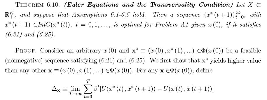
as the difference of the objective function between the feasible sequences x* and x.
From Assumptions 6.2 and 6.5, U is continuous, concave, and differentiable. By definition of a concave function, we have 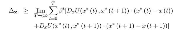
We now illustrate how the tools that have been developed so far can be used in the context of the problem of optimal growth, which will be further discussed in Section 6.6.
EXAMPLE 6.4. Consider the following optimal growth, with log preferences, Cobb-Douglas technology and full depreciation of capital stock
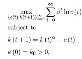
where, as usual, β ∈ (0,1), k denotes the capital-labor ratio (capital stock), and the resource constraint follows from the production function written in per capita terms.
This is one of the canonical examples which admits an explicit-form characterization. To derive this, let us follow Example 6.1 and set up the maximization problem in its recursive form as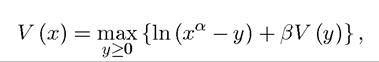
with x corresponding to today’s capital stock and y to tomorrow’s capital stock. Our main objective is to find the policy function y = π (x), which determines tomorrow’s capital stock as a function of today’s capital stock. Once this is done, we can easily determine the level of consumption as a function of today’s capital stock from the resource constraint.
It can be verified that this problem satisfies Assumptions 6.1-6.5. The only non-obvious feature here is whether x and y indeed belong to a compact set. The argument used in Section 6.6 for Proposition 6.1 can be used to verify that this is the case, and we will not repeat the argument here.
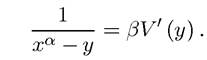
Consequently, Theorems 6.1-6.6 apply. In particular, since V (∙) 239is differentiable, the Euler equation for the one-dimensional case, (6.22), implies
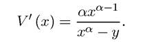
The envelope condition, (6.23), gives:
Thus using the notation y = π (x) and combining these two equations, we have 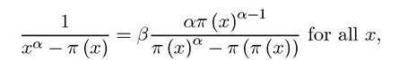 which is a functional equation in a single function, π (x). There are no straightforward ways of solving functional equations, but in most cases guess-and-verify type methods are most fruitful. For example in this case, let us conjecture that

Substituting for this in the previous expression, we obtain
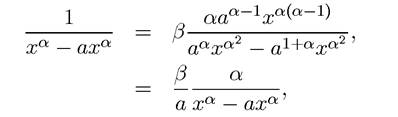
which implies that, with the policy function (6.28), a = βα satisfies this equation. Recall from Corollary 6.1 that, under the assumptions here, there is a unique policy function. Since we have established that the function
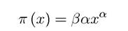
satisfies the necessary and sufficient conditions (Theorem 6.10), it must be the unique policy function. This implies that the law of motion of the capital stock is
(6.28)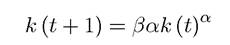
and the optimal consumption level is
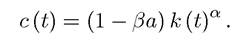
Exercise 6.7 continues with some of the details of this example, and also shows how the optimal growth equilibrium involves a sequence of capital-labor ratios converging to a unique steady state.
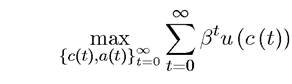
Finally, we now have a brief look at the intertemporal utility maximization problem of a consumer facing a certain income sequence.
EXAMPLE 6.5. Consider the problem of an infinitely-lived consumer with instantaneous utility function defined over consumption u (c), where u : is strictly increasing, contin
uously differentiable and strictly concave. The individual discounts the future exponentially with the constant discount factoι He also faces a certain (nonnegative) labor
240
income stream of {w (t)}t=0, and moreover starts life with a given amount of assets a (0). He receives a constant net rate of interest r > 0 on his asset holdings (so that the gross rate of return is 1 + r). To start with, let us suppose that wages are constant, that is, w (t) = w.
Then, the utility maximization problem of the individual can be written as
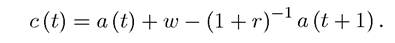
subject to the flow budget constraint

with a (0) > 0 given. In addition, we impose the assumption that the individual cannot have a negative asset holdings, so a (t) ≥ 0 for all t. This example is one of the most common applications of dynamic optimization in economics. Unfortunately, the reader will notice that the feasible set for the state variable a (t) is not necessarily compact, so the theorems developed so far cannot be directly applied to this problem. One way of proceeding is to strengthen these theorems, so that they cover situations in which the feasible set (X in terms of the notation above) is potentially unbounded. While such a strengthening is possible, it requires additional arguments. An alternative approach is to make use of the economic structure of the model. In particular, the following method works in general (but not always, see Exercise 6.13). Let us choose some a and limit a (t) to lie in the set [0, α]. Solve the problem and then verify that indeed a (t) is in the interior of this set. In this example, we can choose a ? a (0) + w/r, which is the sum of the net present discounted value of the labor earnings of the individual and his initial wealth, and will be assumed to be finite below. This strategy of finding an upper bound for the state variable and thus ensuring that it will lie in a compact set is used often in applications.
A couple of additional comments are useful at this point. First the budget constraint could have been written alternatively as a (t + 1) = (1 + r) a (t) + w — c (t). The difference between these two alternative budget constraints involes the timing of interest payments. The first one presumes that the individual starts the period with assets a (t), then receives his labor income, w (t), and then consumes c (t). Whatever is left is saved for the next date and earns the gross interest rate (1 + r). In this formulation, a (t) refers to asset holdings at the beginning of time t. The alternative formulation instead interprets a (t) as asset holdings at the end of time t. The choice between these two formulations has no bearing on the results. Observe also that the flow budget constraint does not capture all of the constraints that individual must satisfy. In particular, an individual can satisfy the flow budget constraint, but run his assets position to -∞. In general to prevent this, we need to impose an additional restriction, for example, that the asset position of the individual 241
does not become “too negative” at infinity. However, here we do not need this additional restriction, since we have already imposed that a (t) ≥ 0 for all t.
Let us also focus on the case where the wealth of the individual is finite, so a (0) < ∞ and w/r < ∞. With these assumptions, let us now write the recursive formulation of the individual’s maximization problem. The state variable is a (t), and consumption can be expressed as
With standard arguments and denoting the current value of the state variable by a and its future value by the recursive form of this dynamic optimization problem can be written as
Clearly u (∙) is strictly increasing in a, continuously differentiable in a and α0 and is strictly concave in a. Moreover, since u (∙) is continuously differentiable in a ∈ (0, a) and the individual’s wealth is finite, V (a (0)) is also finite. Thus all of the results from our analysis above, in particular Theorems 6.1-6.6, apply and imply that V (a) is differentiable and a continuous solution a0 = π (a) exists. Moreover, we can use the Euler equation (6.19), or its more specific form (6.22) for one-dimensional problems to characterize the optimal consumption plan. In particular,
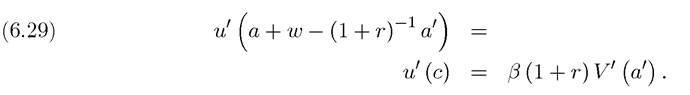
This important equation is often referred to as the “consumption Euler” equation. It states that the marginal utility of current consumption must be equal to the marginal increase in the continuation value multiplied by the product of the discount factor, β, and the gross rate of return to savings, (1 + r). It captures the essential economic intuition of dynamic programming approach, which reduces the complex infinite-dimensional optimization problem to one of comparing today to “tomorrow”. Naturally, the only difficulty here is that tomorrow itself will involve a complicated maximization problem and hence tomorrow’s value function and its derivative are endogenous. But here the envelope condition, (6.23), again comes to our rescue and gives us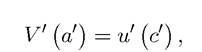
where c0 refers to next period’s consumption. Using this relationship, the consumption Euler equation becomes

This form of the consumption Euler equation is more familiar and requires the marginal utility of consumption today to be equal to the marginal utility of consumption tomorrow multiplied 242
by the product of the discount factor and the gross rate of return. Since we have assumed that β and (1 + r) are constant, the relationship between today’s and tomorrow’s consumption never changes. In particular, since is assumed to be continuously differentiable and strictly concave,
 always exists and is strictly decreasing. Therefore, the intertemporal consumption maximization problem implies the following simple rule:
The remarkable feature is that these statements have been made without any reference to the initial level of asset holdings a (0) and the wage rate w. It turns out that these only determine the initial level of consumption. The “slope” of the optimal consumption path is independent of the wealth of the individual. Exercise 6.12 asks you to determine the level of initial consumption using the transversality condition and the intertemporal budget constraint, while Exercise 6.13 asks you to verify that whenever r ≤ β — 1, a (t) ∈ (0, d) for all t (so that the artificial bounds on asset holdings that I imposed have no bearing on the results).
The problem so far is somewhat restrictive, because of the assumption that wages are constant over time. What happens if instead there is an arbitrary sequence of wages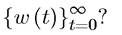
Let us assume that these are known in advance, so that there is no uncertainty. Under this assumption, all of the results derived in this example, in particular, the characterization in (6.31), still apply, but some additional care is necessary, since in this case the budget constraint of the individual, thus the constraint correspondence G in terms of the general formulation above, is no longer “autonomous” (independent of time). In this case, two approaches are possible. The first is to introduce an additional state variable. For example, one can introduce the net present discounted value of future labor earnings,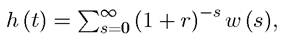
as an additional state variable. In this case, the budget constraint of the individual can be written as

and a similar analysis can be applied with the value function defined over two state variables, V (a, h). This approach is economically meaningful, since the net present discounted value of future earnings is a relevant state variable. But it does not always solve our problems. First, h (t) is now a state variable that has its own non-autonomous evolution (rather than being directly controlled by the individual), so our previous analysis needs to be modified. Second, in many problems, it is difficult to find an economically meaningful additional state variable. Fortunately, however, one can directly apply Theorem 6.10, even when Theorems 6.1-6.6 do not hold. Exercise 6.11 contains the generalization of Theorem 6.10 that enables us to do that, and Exercise 6.12 applies this result to the consumption problem with a time-varying 243
sequence of labor income {w (t)}∞=θ∙ It also shows that the exact shape of this labor income sequence has no effect on the slope or level of the consumption profile.
6.5.2. Dynamic Programming Versus the Sequence Problem. To get more insights into dynamic programming, let us return to the sequence problem. Also, let us suppose that x is one dimensional and that there is a finite horizon T. Then the problem becomes
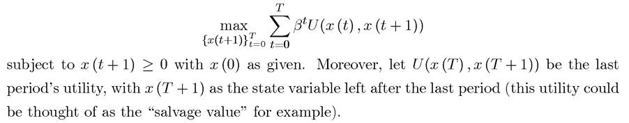
In this case, we have a finite-dimensional optimization problem and we can simply look at first-order conditions. Moreover, let us again assume that the optimal solution lies in the interior of the constraint set, i.e., x* (t) > 0, so that we do not have to worry about boundary conditions and complementary-slackness type conditions. Given these, the first- order conditions of this finite-dimensional problem are exactly the same as the above Euler equation. In particular, we have

which are identical to the Euler equations for the infinite-horizon case. In addition, for x (T + 1), we have the following boundary condition

Intuitively, this boundary condition requires that x* (T + 1) should be positive only if an interior value of it maximizes the salvage value at the end. To provide more intuition for this expression, let us return to the formulation of the optimal growth problem in Example 6.1.
EXAMPLE 6.6. Recall that in terms of the optimal growth problem, we have

with x (t) = k (t) and x (t + 1) = k (t + 1). Suppose we have a finite-horizon optimal growth problem like the one discussed above where the world comes to an end at date T. Then at the last date T, we have
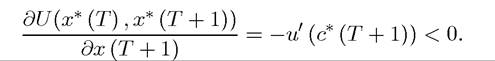
From (6.32) and the fact that U is increasing in its first argument (Assumption 6.4), an optimal path must have k* (T + 1) = x* (T + 1) = 0. Intuitively, there should be no capital left at the end of the world. If any resources were left after the end of the world, utility could be improved by consuming them either at the last date or at some earlier date.
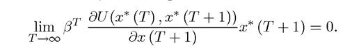
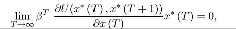
Now, heuristically we can derive the transversality condition as an extension of condition (6.32) to T → ∞. Take this limit, which implies
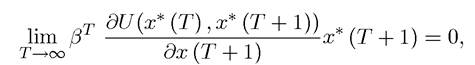
Moreover, as T → ∞, we have the Euler equation
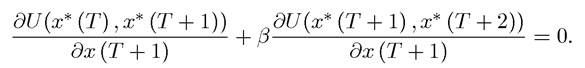
Substituting this relationship into the previous equation, we obtain
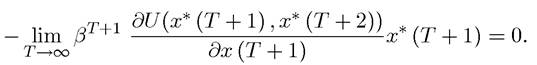
Canceling the negative sign, and without loss of any generality, changing the timing:
which is exactly the transversality condition in (6.26). This derivation also highlights that alternatively we could have had the transversality condition as
which emphasizes that there is no unique transversality condition, but we generally need a boundary condition at infinity to rule out variations that change an infinite number of control variables at the same time. A number of different boundary conditions at infinity can play this role. We will return to this issue when we look at optimal control in continuous time.
6.6.