Optimal Growth in Discrete Time

We are now in a position to apply the methods developed so far to characterize the solution to the standard discrete time optimal growth problem introduced in the previous chapter.

Recall the optimal growth problem for a one-sector economy admitting a representative household with instantaneous utility function u and discount factor β ∈ (0,1). This can be written as

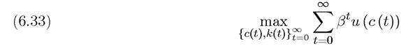
subject to

with the initial capital stock given by k (0).

We continue to make the standard assumptions on the production function as in Assump­tions 1 and 2. In addition, we assume that:

Assumption 30.i is continuously differentiable and strictly concave for

c ∈ [0, ∞).

This is considerably stronger than what we need. In fact, concavity or even continuity is enough for most of the results. But this assumption helps us avoid inessential technical details. The lower bound on consumption is imposed to have a compact set of consumption possibilities. We refer to this as Assumption 3' to distinguish it from the very closely related Assumption 3 that will be introduced and used in Chapter 8 and thereafter.

The first step is to write the optimal growth problem as a (stationary) dynamic program­ming problem. This can be done along the lines of the above formulations. In particular, let the choice variable be next date’s capital stock, denoted by s.

(6.34) implies that current consumption is given by c = f (k) + (1 — δ) k — s, and thus we can write the open growth problem in the following recursive form:

(6.35)

where G (k) is the constraint correspondence, given by the interval which imposes that consumption cannot fall below c and that the capital stock cannot be negative.

It can be verified that under Assumptions 1, 2 and 3', the optimal growth problem satisfies Assumptions 6.1-6.5 of the dynamic programming problems. The only non-obvious feature is that the level of consumption and capital stock belong to a compact set. To verify that this is the case, note that the economy can never settle into a level of capital-labor ratio greater than k, de fined by

since this is the capital-labor ratio that would sustain itself when consumption is set equal to 0. If the economy starts with k (0) < ê, it can never exceed ê. If it starts with k (0) > ê, it can never exceed k (0). Therefore, without loss of any generality, we can restrict consumption and capital stock to lie in the compact set, where

Consequently, Theorems 6.1-6.6 immediately apply to this problem and we can use these results to derive the following proposition to characterize the optimal growth path of the one-sector infinite-horizon economy.

PROPOSITION 6.1. Given Assumptions 1, 2 and 3', the optimal growth model as specified in (6.33) and (6.34) has a solution characterized by the value function V (k) and consumption 246

function c (k).

Proof. Optimality of the solution to the value function (6.35) for the problem (6.33) and (6.34) follows from Theorems 6.1 and 6.2. That V (k) exists follows from Theorem 6.3, and the fact that it is increasing and strictly concave, with the policy correspondence being a policy function follows from Theorem 6.4 and Corollary 6.1.

Thus we only have to show that s (k) is nondecreasing. This can be proved by contradic­tion. Suppose, to arrive at a contradiction, that s (k) is decreasing, i.e., there exists k and k⁰ > k such that s (k) > s (k⁰). Since k⁰ > k, s (k) is feasible when the capital stock is k⁰. Moreover, since, by hypothesis, s (k) > s (k⁰), s (k⁰) is feasible at capital stock k.

By optimality and feasibility, we must have:

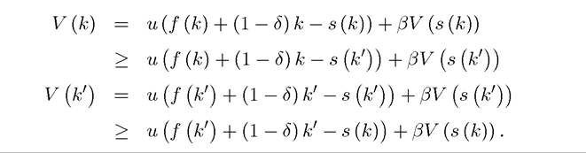
Combining and rearranging these, we have

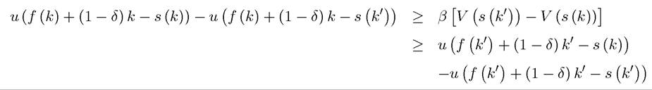
Or denoting z ? f (k) + (1 — δ) k and x ? s (k) and similarly for z' and x', we have

But clearly,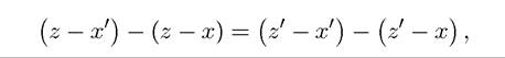

which combined with the fact that z⁰ > z (since k⁰ > k) and x > x' by hypothesis, and that u is strictly concave and increasing implies

contradicting (6.36). This establishes that s (k) must be nondecreasing everywhere. ?

In addition, Assumption 2 (the Inada conditions) imply that savings and consumption levels have to be interior, thus Theorem 6.6 applies and immediately establishes:

Proposition 6.2.

Consequently, from Theorem 6.10, we can look at the Euler equations. The Euler equation from (6.35) takes the simple form:

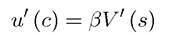
where s denotes the next date’s capital stock. Applying the envelope condition, we have

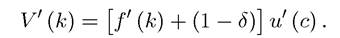
Consequently, we have the familiar condition

As before, a steady state is as an allocation in which the capital-labor ratio and consumption do not depend on time, so again denoting this by *, we have the steady state capital-labor ratio as

which is a remarkable result, because it shows that the steady state capital-labor ratio does not depend on preferences, but simply on technology, depreciation and the discount factor. We will obtain an analog of this result in the continuous-time neoclassical model as well.

Moreover, since f (∙) is strictly concave, k* is uniquely defined. Thus we have

Proposition 6.3. In the neoclassical optimal growth model specified in (6.33) and (6.34) with Assumptions 1, 2 and 30, there exists a unique steady-state capital-labor ratio k* given by (6.38), and starting from any initial k (0) > 0, the economy monotonically converges to this unique steady state, i.e.,then the equilibrium capital stock sequence

and if k (0) > ê*, then the equilibrium capital stock sequence

Proof.

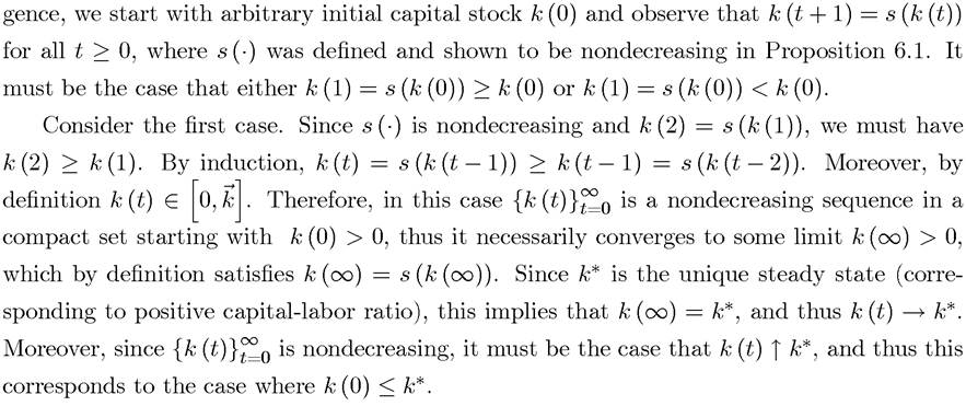
Next consider the case in which k (1) = s (k (0)) < ê (0). The same argument as above

Consequently, in the optimal growth model there exists a unique steady state and the economy monotonically converges to the unique steady state, for example by accumulating more and more capital (if it starts with a too low capital-labor ratio).

We can also show that consumption also monotonically increases (or decreases) along the path of adjustments to the unique-steady state:

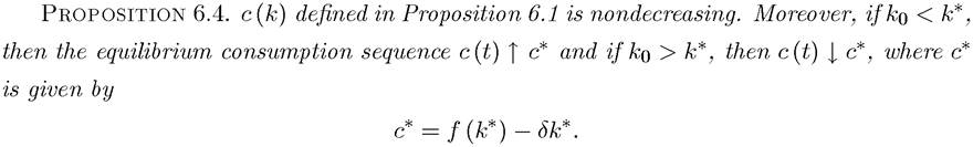
Proof. See Exercise 6.16.

This discussion illustrates that the optimal growth model is very tractable, and we can easily incorporate population growth and technological change as in the Solow growth model. There is no immediate counterpart of a saving rate, since this depends on the utility function. But interestingly and very differently from the Solow growth model, the steady state capital­labor ratio and steady state income level do not depend on the saving rate anyway.

We will return to all of these issues, and provide a more detailed discussion of the equi­librium growth in the context of the continuous time model. But for now, it is also useful to see how this optimal growth allocation can be decentralized, i.e., in this particular case we can use the Second Welfare Theorem to show that the optimal growth allocation is also a competitive equilibrium.

Finally, it is worth noting that results concerning the convergence behavior of the optimal growth model are sometimes referred to as the “Turnpike Theorem ”. This term is motivated by the study of finite-horizon versions of this model. In particular, suppose that the economy ends at some date T > 0. How do optimal growth and capital accumulation look like in this economy? The early literature on optimal growth showed that as T → ∞, the optimal capital­labor ratio sequence {k (t)}(L₀ would become arbitrarily close to k* as defined by (6.38), but then in the last few periods, it would sharply decline to zero to satisfy the transversality condition (recall the discussion of the finite-horizon transversality condition in Section 6.5).

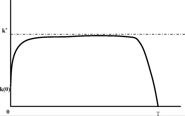
Figure 6.1. Turnpike dynamics in a finite-horizon (T-periods) neoclassical growth model starting with initial capital-labor ratio k (0).

The path of the capital-labor ratio thus resembles a turnpike approaching a highway as shown in Figure 6.1 (see Exercise 6.17).

6.7.