Optimal Growth

Motivated by the discussion in the previous section let us start with an economy char­acterized by an aggregate production function, and a representative household. The optimal growth problem in this context refers to characterizing the allocation of resources that max­imizes the utility of the representative household.

is the utility function of the representative household. The objective function represents the discounted sum of this utility function. The constraint (5.24) is also straightforward to understand; total output per capita produced with capital-labor ratio k (t), f (k (t)), together with a fraction 1 — δ of the capital that is undepreciated make up the total resources of the economy at date t. Out of this resources c (t) is spent as consumption per capita c (t) and the rest becomes next period’s capital-labor ratio, k (t + 1).

The optimal growth problem imposes that the social planner chooses an entire sequence of consumption levels and capital stocks, only subject to the resource constraint, (5.24). There are no additional equilibrium constraints. The initial level of capital stock k (0) > 0 has been specified as one boundary condition. But in contrast to the basic Solow model, the solution to this problem involves two, not one, dynamic (difference or differential) equations, and thus necessitates two boundary conditions.

This maximization problem can be solved in a number of different ways, for example, by setting up an infinite-dimensional Lagrangian. But the most convenient and common way of approaching it is by using dynamic programming.

It is also useful to note that even if we wished to bypass the Second Welfare Theorem and directly solve for competitive equilibria, we would have to solve a problem similar to the maximization of (5.23) subject to (5.24). In particular, to characterize the equilibrium, we would need to start with the maximizing behavior of households. Since the economy admits a representative household, we only need to look at the maximization problem of this household. Assuming that the representative household has one unit of labor supplied

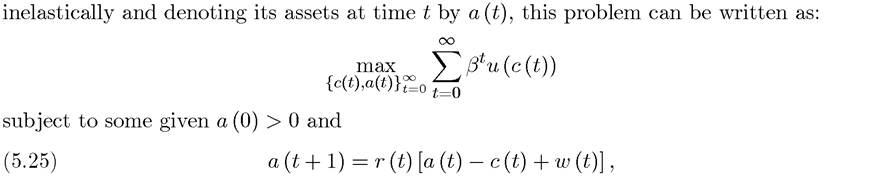
where r (t) is the rate of return on assets and w (t) is the equilibrium wage rate (and thus the wage earnings of the representative household). Market clearing then requires that a (t) = k (t). The constraint, (5.25) is the flow budget constraint, meaning that it links tomorrow’s assets to today’s assets. Here we need an additional condition so that this flow budget constraint eventually converges (so that a (t) should not go to negative infinity). This can be ensured by imposing a lifetime budget constraint. Since a flow budget constraint in the form of (5.25) is both more intuitive and often more convenient to work with, we will not work with the lifetime budget constraint, but augment the flow budget constraint with a limiting

condition, which will be introduced and discussed below.

The formulation of the optimal growth problem in continuous time is very similar and takes the form

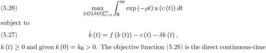
analog of (5.23), and (5.27) gives the resource constraint of the economy, similar to (5.24) in discrete time. Once again, this problem lacks one boundary condition which will come from the transversality condition. The most convenient way of characterizing the solution to this problem is via optimal control theory. Dynamic programming and optimal control theory will be discussed briefly in the next two chapters.

5.10.