Sequential Trading
A final issue that is useful to discuss at this point relates to sequential trading. Standard general equilibrium models assume that all commodities are traded at a given point in time— and once and for all.
That is, once trading takes place at the initial date, there is no more trade or production in the economy. This may be a good approximation to reality when different commodities correspond to different physical goods. However, when different commodities 190correspond to the same good in different time periods or in different states of nature, trading at a single point is much less reasonable. Models of economic growth typically assume that trading takes place at different points in time. For example, in the Solow growth model of Chapter 2, we envisaged firms hiring capital and labor at each t. Does the presence of sequential trading make any difference to the insights of general equilibrium analysis? If the answer to this question were yes, then the applicability of the lessons from general equilibrium theory to dynamic macroeconomic models would be limited. Fortunately, in the presence of complete markets, sequential trading gives the same result as trading at a single point in time.
More explicitly, the Arrow-Debreu equilibrium of a dynamic general equilibrium model involves all the households trading at a single market at time t = 0 and purchasing and selling irrevocable claims to commodities indexed by date and state of nature. This means that at time t = 0, households agree on all future trades (including trades of goods that are not yet produced). Sequential trading, on the other hand, corresponds to separate markets opening at each t, and households trading labor, capital and consumption goods in each such market at each period. Clearly, both for mathematical convenience and descriptive realism, we would like to think of macroeconomic models as involving sequential trading, with separate markets at each date.
The key result concerning the comparison of models with trading at a single point in time and those with sequential trading is due to Kenneth Arrow (1964). Arrow’s focus was on trading across states of nature. However, his results also imply that with complete markets (and time-consistent preferences), trading at a single point in time and sequential trading are equivalent. The easiest way of seeing this is to consider the Arrow securities already discussed in Chapter 2. (Basic) Arrow Securities provide an economical means of transferring resources across different dates and different states of nature. Instead of completing all trades at a single point in time, say at time t = 0, households can trade Arrow securities and then use these securities to purchase goods at different dates or after different states of nature have been revealed. While Arrow securities are most useful when there is uncertainty as well as a temporal dimension, for our purposes it is sufficient to focus on the transfer of resources across different dates.
The reason why sequential trading with Arrow securities achieves the same result as trading at a single point in time is simple: by the definition of a competitive equilibrium, households correctly anticipate all the prices that they will be facing at different dates (and in different states of nature) and purchase sufficient Arrow securities to cover the expenses that they will incur once the time to trade comes. In other words, instead of buying claims at time units of commodity j = 1,...,N at date t' at prices
 it is
it is
sufficient for household h to have an income of and know that it can purchase
as many units of each commodity as it wishes at time t' at the price vector
This result can be stated in a slightly more formal manner.
Let us consider a dynamic exchange economy running across periods t = 0,1,...,T, possibly with T = ∞ (with the convention that when T = ∞, all the summations are assumed to take finite values). Nothing here depends on the assumption that we are focusing on an exchange economy, but suppressing production simplifies notation. Imagine that there are N goods at each date, denoted by (xgt,...,XNt), and let the consumption of good j by household h at time t be denoted by Suppose that these goods are perishable, so that they are indeed consumed at time t. Denote the set of households by H and suppose that each household h ∈ H has a vector of endowment
 at time t, and preferences given by the time-separable function of
 the form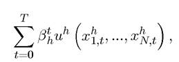
for some βh ∈ (0,1). These preferences imply that there are no externalities and preferences are time-consistent. I also assume that all markets are open and competitive.
Let an Arrow-Debreu equilibrium be given by (p*, x*), where x* is the complete list of consumption vectors of each household h ∈ H, that is,
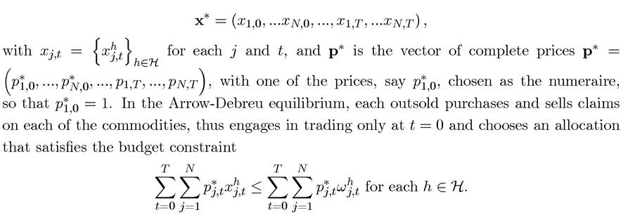
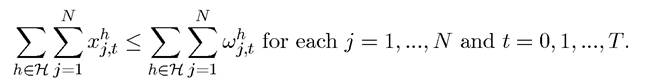
Market clearing then requires
In the equilibrium with sequential trading, markets for goods dated t open at time t. Instead, there are T bonds—Arrow securities—that are in zero net supply and can be traded among the households at time t = 0. The bond indexed by t pays one unit of one of the goods, say good j = 1 at time t. Let the prices of bonds be denoted by (qι,...,qτ), again expressed in units of good j = 1 (at time t = 0).
This implies that a household can purchase a unit of bond t at time 0 by paying qt units of good 1, and in return, it will receive one unit of good 1 at time t (or conversely can sell short one unit of such a bond) The purchase of bond t by household h is denoted by and since each bond is in zero net supply, market clearing requires that
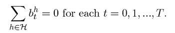
Notice that this specification assumes that there are only T bonds (Arrow securities). More generally, I could have introduced additional bonds, for example, bonds traded at time t > 0 for delivery of good 1 at time t' > t. This restriction to only T bonds is without loss of any generality (see Exercise 5.10).
Sequential trading corresponds to each individual using their endowment plus (or minus) the proceeds from the corresponding bonds at each date t. Since there is a market for goods at each t, it turns out to be convenient (and possible) to choose a separate numeraire for each date t, and let us again suppose that this numeraire is good 1, so that pj*t = 1 for all t. Therefore, the budget constraint of household h ∈ H at time t, given the equilibrium price vector for goods and bonds,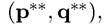 can be written as:
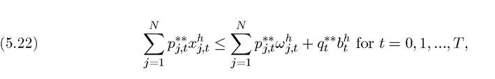
with the normalization that qθ* = 1. Let an equilibrium of the sequential trading economy be denoted by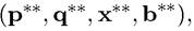 where once again
 and x** denote the entire lists of
prices and quantities of consumption by each household, and and
and denote the vector of bond prices and bond purchases by each household.
Proof. See Exercise 5.9. ?
This theorem implies that all the results concerning Arrow-Debreu equilibria apply to economies with sequential trading. In most of the models studied in this book (except in the context of endogenous financial markets), the focus will be on economies with sequential trading and assume that there exist Arrow securities to transfer resources across dates. These securities might be riskless bonds in zero net supply, or in models without uncertainty, this role will typically be played by the capital stock. I also follow the approach leading to Theorem 5.8 and normalize the price of one good at each date to 1. This implies that in economies with a single consumption good, like the Solow or the neoclassical growth models, the price of the consumption good in each date will be normalized to 1 and the interest rates will directly give the intertemporal relative prices. This is the justification for focusing on interest rates as the key relative prices in macroeconomic (economic growth) models.
5.9.