The Maximum Principle: A First Look

7.2.1. The Hamiltonian and the Maximum Principle. By analogy with the La­grangian, a much more economical way of expressing Theorem 7.2 is to construct the Hamil­tonian:^[11]

Since f and g are continuously differentiable, so is H.

Theorem 7.4. (Simplified Maximum Principle) Consider the problem of maximizing (7.1) subject to (7.2) and (7.3), with f and g continuously differentiable. Suppose that this problem has an interior continuous solution y(t) ∈Inty (t) and X (t) ∈IntX (t). Then, there exists a continuously differentiable function λ (t) such that the optimal control y (t) and the corresponding path of the state variable X (t) satisfy the following necessary conditions: x (0) = xo,

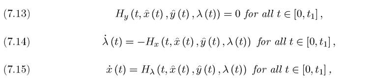
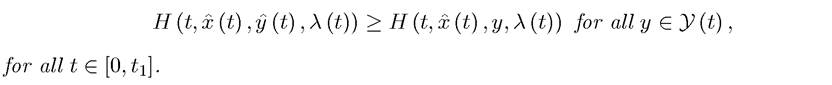
and λ (tι) = 0, with the Hamiltonian H (t, x, y, λ) given by (7.12). Moreover, the Hamiltonian H (t,x,y,λ) also satisfies the Maximum Principle that

For notational simplicity, in eq. (7.15), I wrote x (t) instead of ^(t) (= ∂^(t) /∂t). The latter notation is rather cumbersome, and I refrain from using it as long as the context makes it clear that x (t) stands for this expression.

Theorem 7.4 is a simplified version of the celebrated Maximum Principle of Pontryagin. The more general version of this Maximum Principle will be given below. For now, a couple of features are worth noting:

(1) As in the usual constrained maximization problems, the optimal solution is char­acterized jointly with a set of “multipliers,” here the costate variable λ (t), and the optimal path of the control and state variables,

(2) Again as with the Lagrange multipliers in the usual constrained maximization prob­lems, the costate variable λ (t) is informative about the value of relaxing the con­straint (at time t).

(3) With this interpretation, it makes sense that λ (tι) = 0 is part of the necessary conditions. After the planning horizon, there is no value to having more x. This is therefore the finite-horizon equivalent of the transversality condition in the previous chapter.

As emphasized above, Theorem 7.4 gives necessary conditions for an interior continuous solution. However, we do not know that such a solution exists. Moreover, even when such a solution exists, it may correspond to a “stationary point” rather than a maximum, or it may be a local rather than a global maximum of the optimization problem. Therefore, a sufficiency result is even more important in this context than in finite-dimensional optimization problems. Sufficiency is again guaranteed by imposing concavity. The following theorem, first proved by Mangasarian, shows that concavity of the Hamiltonian ensures that conditions (7.13)-(7.15) are not only necessary but also sufficient for a maximum.

Theorem 7.5. (Mangasarian’s Sufficiency Conditions) Consider the problem of maximizing (7.1) subject to (7.2) and (7.3), with f and g continuously differentiable. Define H (t,x,y, λ) as in (7.12), and suppose that an interior continuous solutionand

exists and satisfies (7.13)-(7.15). Suppose also that given the resulting costate variable λ (t), H (t, x, y, λ) is jointly concave in (x, y) for all t ∈ [0,tι], then the y (t) and the corresponding x(t) achieve a global maximum of (7.1). Moreover, if H (t,x,y,λ) is strictly jointly concave in (x,y) for all t ∈ [0,tι], then theis the unique solution to

(7.1).

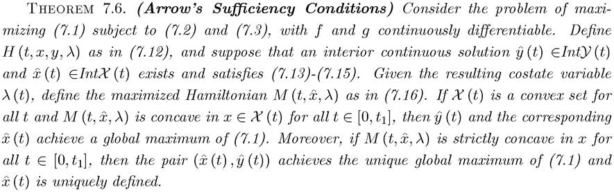
The proof of Theorem 7.5 follows from the proof of Theorem 7.6 and is discussed after the next theorem.^[12] The next result, Theorem 7.6, which was first derived by Arrow, weakens the condition that H (t, x,y,λ) is jointly concave in (x,y). Before stating this result, let us

define the maximized Hamiltonian as

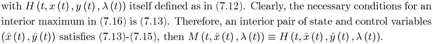
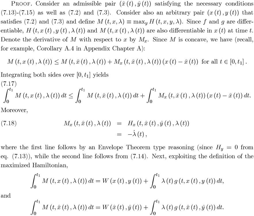
Equation (7.17) together with (7.18) then implies

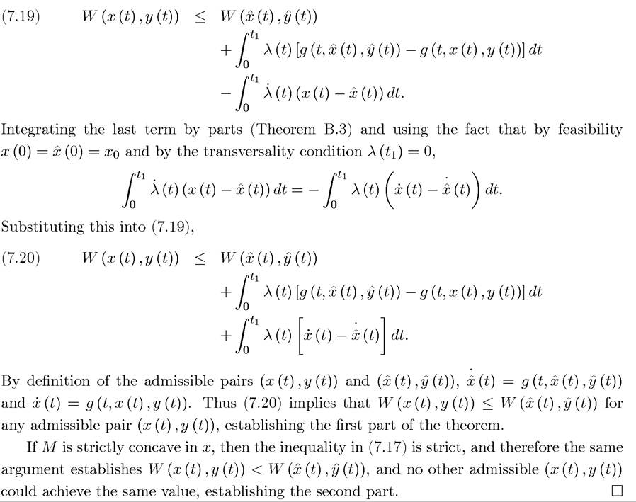
Given Theorem 7.6, the proof of Theorem 7.5 follows as a direct corollary, since if a function H (t, x, y, λ) is jointly [strictly] concave in (x, y), then M (t, x, λ) ? maxy H (t, x, y, λ) is [strictly] concave in x (see Exercise 7.7). Nevertheless, in many applications it may be easier to verify that H (t,x,y,λ) is jointly concave in (x,y) rather than looking at the maximized Hamiltonian. Moreover, in some problems M (t, x, λ) may be concave in x, while H (t, x, y, λ) is concave in (x, y) and strictly concave in y, and this information may be useful in establishing uniqueness. However, to economize on space, I focus on sufficiency theorems along the lines of Theorem 7.6.

Sufficiency results as in Theorems 7.5 and 7.6 play an important role in the applications of optimal control. They ensure that an admissible pair (x (t),y (t)) that satisfies the necessary conditions specified in Theorem 7.4 and the sufficiency conditions in either Theorem 7.5 or Theorem 7.6 is indeed an optimal solution. This is important, since without the sufficiency results, Theorem 7.4 does not tell us that there exists an interior continuous solution, thus an admissible pair that satisfies the conditions of Theorem 7.4 may not be optimal or an optimal solution may not satisfy these “necessary conditions” (because it is not interior or continuous).

(satisfying the necessary conditions for an interior continuous solution) corresponds to a global maximum or a unique global maximum.

One difficulty in verifying that the conditions in Theorem 7.5 and Theorem 7.6 are sat­isfied is that neither the concavity nor convexity of the g (∙) function would guarantee the concavity of the Hamiltonian unless we know something about the sign of the costate variable λ (t). Nevertheless, in many economically interesting situations, we can ascertain that the costate variable λ (t) is everywhere positive. For example,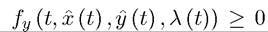and

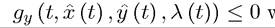rill be sufficient to ensure that λ (t) ≥ 0. Once we know that λ (t) is nonnegative, checking the sufficiency conditions is straightforward, especially when f and g are concave functions.

7.2.2. Generalizations. The above theorems can be generalized to the case in which the state variable and the controls are vectors and also to the case in which there are other constraints. The constrained case requires constraint qualification conditions as in the stan­dard finite-dimensional optimization case (see, e.g., Theorems A.30 and A.31 in Appendix Chapter A). These are slightly more messy to express. Since I make no use of the constrained maximization problems (except in Exercise 10.7 in Chapter 10), I only discuss constrained problems briefly in Exercise 7.10.

The vector-valued theorems are direct generalizations of the ones presented above and are useful in growth models with multiple capital goods. In particular, let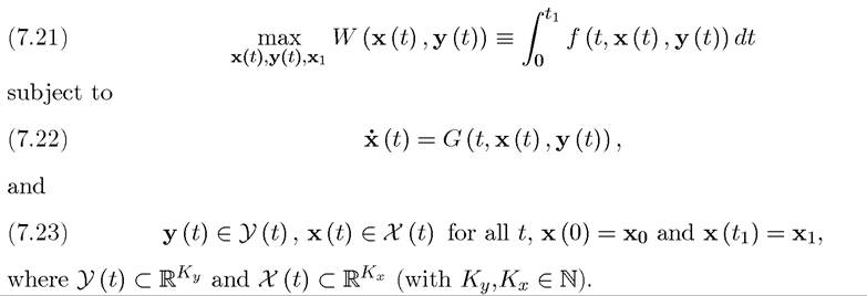

Theorem 7.7. (Maximum Principle for Multivariate Problems) Consider the problem of maximizing (7.21) subject to (7.22) and (7.23), with f and G continuously dif­ferentiable, has an interior continuous solutionLet

H (t, x, y, λ) be given by

where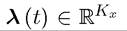(and λ∙G denotes the inner product of the vectors λ and G).

optimal controland the corresponding path of the state variable x (t) satisfy the following

necessary conditions: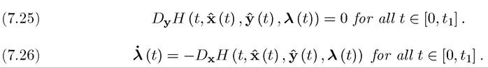

Proof. See Exercise 7.11. ?

Note also that various conditions in this theorem can be relaxed. For example, the conditions thatare not necessary, and when either the state

or the control variables take boundary values, there may be jumps in the control variables and the Hamiltonian may not be differentiable everywhere (see below). However, recall that all we require is a piecewise continuous (vector-valued) function y (t), so that this does not create major problems. Since in most economic applications both state and control variables will be interior and the corresponding Hamiltonian will be differentiable everywhere, the form of Theorem 7.7 stated here is sufficient for most problems of interest.

Moreover, the sufficiency conditions for a maximum provided above also have straight­forward generalizations, which are presented next.

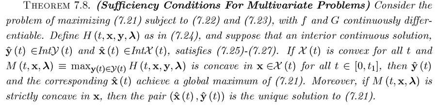
Proof. See Exercise 7.12. ?

7.2.3. Limitations. The limitations of the results presented so far are obvious. First, a continuous and interior solution to the optimal control problem has been assumed. Second, and equally important, the analysis has focused on the finite-horizon case whereas analysis of growth models requires us to solve infinite-horizon problems. To deal with both of these issues, we need to look at the more modern theory of optimal control. This is done in the next section.

7.3.