Introduction to Stationary Dynamic Programming

Let us consider the stationary form of Problem A0,

Problem A1 :

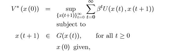
where again β ∈ [0,1), and now the constraint correspondence and the instantaneous payoff functions take the formThis problem is stationary because

U and G do not explicitly depend on time.

Problem A1, like Problem A0, corresponds to the sequence problem; it involves choosing an infinitesequenc501" class="lazyload" data-src="/files/uch_group77/uch_pgroup317/uch_uch7365/image/image501.jpg">

sides of eq. (6.1) and is thus defined recursively. The functional equation in Problem A2 is also called the Bellman equation, after Richard Bellman, who was the first to introduce the dynamic programming formulation.

At first sight, the recursive formulation might not appear as a great advance over the sequence formulation. After all, functions might be trickier to work with than sequences. Nevertheless, it turns out that the functional equation of dynamic programming is easy to work with in many instances. In applied mathematics and engineering, it is favored because it is computationally convenient. In economics, perhaps the major advantage of the recursive formulation is that it often gives better economic insights, similar to the logic of comparing today to tomorrow. In particular, U (x,y^) is the“ return for today” and βV (y) is the continuation return from the next date onwards, equivalent to the “return for tomorrow”. Consequently, in many applications we can use our intuitions from two-period maximization or economic problems. Finally, in some special but important cases, the solution to Problem A2 is simpler to characterize analytically than the corresponding solution of the sequence problem, Problem A1.

In fact, the form of Problem A2 suggests itself naturally from the formulation Problem A1. Suppose Problem A1 has a maximum starting at x (0) attained by the optimal sequence 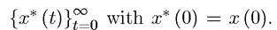Then, under some relatively weak technical conditions, we have that

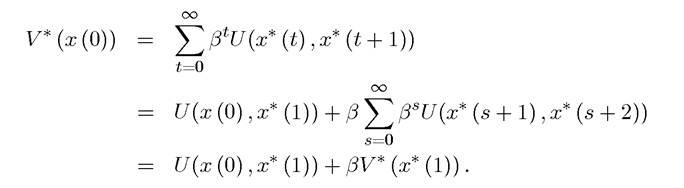
This equation encapsulates the basic idea of dynamic programming, the Principle of Opti­mality, which will be stated more formally in Theorem 6.2.

Essentially, an optimal plan can be broken into two parts, what is optimal to do today, and the optimal continuation path. Dynamic programming exploits this principle and provides us with a set of powerful tools to analyze optimization in discrete-time infinite-horizon problems.

As noted above, the particular advantage of this formulation is that the solution can be represented by a time invariant policy function (or policy mapping), 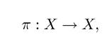determining which value of x (t + 1) to choose for a given value of the state variable x (t). In general, there will be two complications: first, a control reaching the optimal value may not exist, which was the reason why I originally used the notation sup; second, the solution to Problem A2 may involve not a policy function, but a policy correspondence, because there may be more than one maximizer for a given state variable. Let us ignore these complications for now and present a heuristic exposition. These issues will be dealt with in greater detail below.

Once the value function V is determined, the policy function is given straightforwardly. In particular, by definition it must be the case that if optimal policy is given by a policy

207

function π (x), then

which is one way of determining the policy function.

The usefulness of the recursive formulation in Problem A2 comes from the fact that there are some powerful tools that not only establish the existence of a solution, but also some of its properties. These tools are also utilized directly in a variety of problems in economic growth, macroeconomics and other areas of economic dynamics.

The next section presents results about the relationship between the solution to the se­quence problem, Problem A1, and the recursive formulation, Problem A2. More importantly, the tool also present a number of results on the concavity, monotonicity and differentiability of the value function V (∙) (and of the value function V * (∙) in Problem A1).

6.3.