Optimal Growth in Discrete Time

Let us now return to the optimal growth problem, introduced in Section 5.9, and use the main results from stationary dynamic programming to obtain a characterization of the optimal growth path of a neoclassical economy.

Recall the optimal growth problem for a one-sector economy admitting a representative household with instantaneous utility function u and discount factor β ∈ (0,1). This can be written as

with the initial capital stock given by k (0) > 0.

The standard assumptions on the production function, Assumptions 1 and 2, are still in effect. In addition, let us impose:

This is considerably stronger than necessary. In fact, concavity or even continuity is enough for most of the results. But this assumption helps us avoid inessential technical details. This assumption is referred to as Assumption 3⁰ to distinguish it from the very closely related Assumption 3 that will be introduced and used in Chapter 8 and thereafter.

239

The first step is to write the optimal growth problem as a (stationary) dynamic program­ming problem. This can be done along the lines of the above formulations. In particular, let the choice variable be next date’s capital stock, denoted by s. Then, the resource constraint (6.44) implies that current consumption is given by c = f (k) + (1 — δ) k — s, and thus the optimal growth problem can be written in the following recursive form:

where G (k) is the constraint correspondence, given by the interval [0,f (k) + (1 — δ) k], which imposes that consumption cannot be negative and that the capital stock cannot be negative.

It can be verified that under Assumptions 1, 2 and 30, the optimal growth problem satisfies Assumptions 6.1-6.5 of the dynamic programming problems. The only non-obvious feature is that the level of consumption and capital stock belong to a compact set. To verify that this is the case, note that the economy can never settle into a level of capital-labor ratio greater than k, de fined by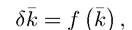

Consequently, Theorems 6.1-6.6 can be directly applied to this problem.

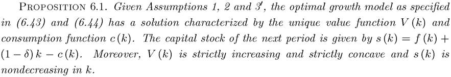
Proof. That the value function (6.45) is a solution to (6.43) and (6.44) follows from Theorems 6.1 and 6.2. That V (k) exists follows from Theorem 6.3, and the fact that it is increasing and strictly concave, with the policy correspondence being a policy function, follows from Theorem 6.4 and Corollary 6.1.

As before, a steady state (of the optimal growth problem) is as an allocation in which the capital-labor ratio and consumption do not depend on time, so again denoting this allocation by *, the steady state capital-labor ratio must satisfy

This is a remarkable result; it shows that the steady-state capital-labor ratio does not depend on household preferences except via the discount factor. In particular, technology, the de­preciation rate and the discount factor fully characterize the steady-state capital-labor ratio. An analog of this result applies in the continuous-time neoclassical model as well.

Proposition 6.3.

Consequently, in the optimal growth model there exists a unique steady state and the economy monotonically converges to the unique steady state, for example by accumulating more and more capital (if it starts with a too low capital-labor ratio).

In addition, consumption also monotonically increases (or decreases) along the path of adjustments to the unique-steady state:

Proof. See Exercise 6.17. ?

This discussion illustrates that the optimal growth model is very tractable and shares many commonalities with the Solow growth model, for example, a unique steady state and global monotonic convergence. There is no immediate counterpart of a saving rate, since the amount of savings depends on the utility function and changes over time, though the discount factor is closely related to the saving rate.

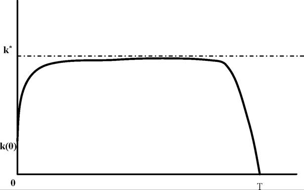
Figure 6.1. Turnpike dynamics in a finite-horizon (T-periods) neoclassical growth model starting with initial capital-labor ratio k (0).

The convergence behavior of the optimal growth model is both important and remarkable in its simplicity. Such convergence results, which were first studied in the context of finite- horizon economies, are sometimes referred to as “Turnpike Theorems ”. To understand the meaning of this term, suppose that the economy ends at some date T > 0. How do optimal growth and capital accumulation look like in this economy? The early literatureon optimal growth showed that as T → ∞, the optimal capital-labor ratio sequencewould

become arbitrarily close to k* as defined by (6.49), but then in the last few periods, it would sharply decline to zero to satisfy the transversality condition (recall the discussion of the finite-horizon transversality condition in Section 6.6). The path of the capital-labor ratio thus resembles a turnpike approaching a highway as shown in Figure 6.1 (see Exercise 6.18).

6.9.