Competitive Equilibrium Growth
Our main interest is not optimal growth, but equilibrium growth. A detailed analysis of competitive equilibrium growth will be presented in Chapter 8. For now a brief discussion of how the competitive equilibrium can be obtained from the optimal growth problem is sufficient.
The Second Welfare Theorem, Theorem 5.7 of the previous chapter, implies that the optimal growth path characterized in the previous section also corresponds to an equilibrium growth path (in the sense that, it can be decentralized as a competitive equilibrium). In fact, since we have focused on an economy admitting a representative household, the most straightforward competitive allocation would be a symmetric one, where all households, each with the instantaneous utility function u (c), make the same decisions and receive the same allocations. I now discuss this symmetric competitive equilibrium briefly.Rather than appealing to the Second Welfare Theorem, a direct argument can also be used to show the equivalence of optimal and competitive growth problems. Suppose that each household starts with an endowment of capital stock Ko, meaning that the initial endowments are also symmetric (recall that there is a mass 1 of households and the total initial endowment of capital of the economy is Ko). The other side of the economy is populated by a large number of competitive firms, which are modeled using the aggregate production function.
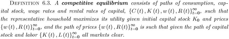
The definition of a competitive equilibrium in this economy is standard.
with a (0) > 0, where a (t) denotes asset holdings at time t and as before, w (t) is the wage income of the household (since labor supply is normalized to 1).
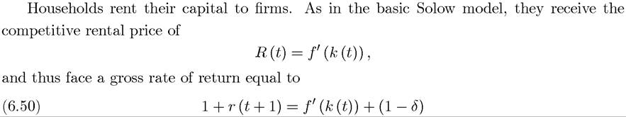
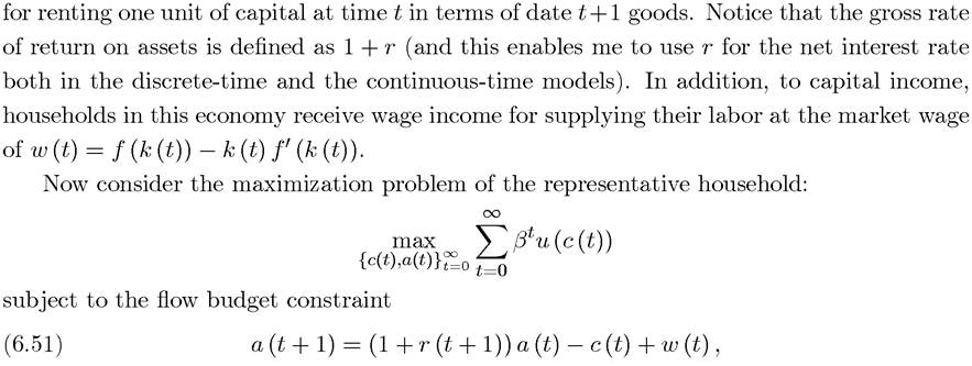
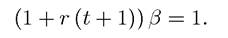
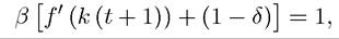
The timing underlying the flow budget constraint (6.51) is that the household rents his capital or asset holdings, a (t), to firms to be used as capital at time t + 1. Out of the proceeds, it consumes and whatever is left, together with its wage earnings, w (t), make up its asset holdings at the next date, a (t + 1). Once again, we impose the natural debt limit, which takes the form of equation (6.41) in the continuation of Example 6.5, and market clearing again implies a (t) = k (t).With an argument identical to that in Example 6.5, the Euler equation for the consumer maximization problem yields

Imposing steady state implies that c (t) = c (t + 1). Therefore, in steady state,
Next, market clearing immediately implies that 1 + r (t + 1) is given by (6.50), so the capitallabor ratio of the competitive equilibrium is given by
The steady state is given by
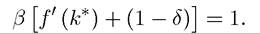
These two equations are identical to eq.’s (6.49) and (6.50), which characterize the solution to the optimum growth problem. A similar argument establishes that the entire competitive equilibrium path is identical to the optimal growth path. Specifically, substituting for 1 + r (t + 1) from (6.50) into (6.52),

which is identical to (6.47). This condition also implies that given the same initial condition, the trajectory of capital-labor ratio in the competitive equilibrium will be identical to the behavior of the capital-labor ratio in the optimal growth path (see Exercise 6.21). This is, of course, exactly what should be expected given the Second (and First) Welfare Theorems.
6.10.