Nonstationary Infinite-Horizon Optimization
6.7.1. Main Results. Let us now return to Problem A0. The possible nonstationarity in this problem makes it considerably more difficult than Problems A1 and A2. Nevertheless, many important economic problems, for example, utility maximization by a household in a dynamic competitive equilibrium corresponds to such a nonstationary problem.
One way of making progress is to introduce additional assumptions on U and G so as to obtain the equivalents of Theorems 6.1-6.6 (see, for example, Exercise 6.14). Nevertheless, existence of solutions and the necessity and sufficiency of Euler equations and the transversality conditions (as in Theorem 6.10) can be established under fairly general conditions. This is the approach I use in this section. In particular, let us again define the set of feasible sequences or plans starting with an initial value x (t) at time t as:
Also denote an element of this set by x [t] = (x (t),x (t + 1),...) ∈Φ(t, x (t)). The key assumptions will be as follows (and they are numbered with reference to Assumptions 6.1-6.5 above):
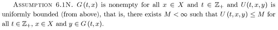
This assumption is again stronger than necessary to establish the results that will follow, but it simplifies the exposition. 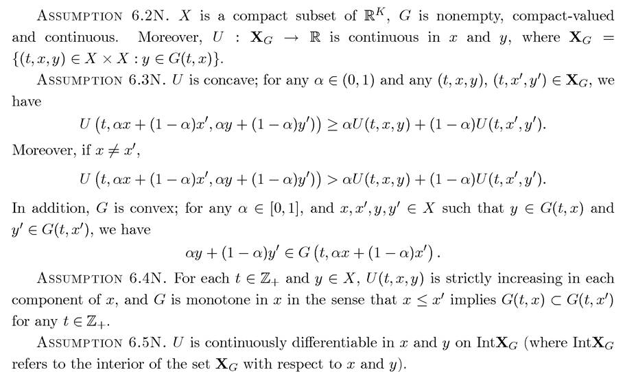
The two key results are the following. The proofs of both theorems are given in the next subsection.
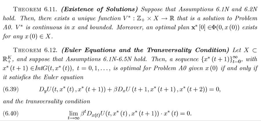
In equation (6.39), as in stationary problems, Dy U denotes the vector of partial derivatives of U with respect to the control vector (its last K arguments), whereas DxU denotes the vector of partial derivatives with respect to the state vector.
In (6.40), “•” again denotes the inner product of the two vectors.These two theorems provide us with the necessary tools to tackle nonstationary discretetime infinite-horizon optimization problems. In particular, Theorem 6.11 ensures that the solution exists and Theorem 6.12 shows that, as in the stationary case, we can simply use the Euler equations and the transversality condition to characterize this solution (as long as it is interior).
6.7.2. Proofs of Theorems 6.11 and 6.12*..
Proof of Theorem 6.11. Since U is uniformly bounded (Assumption 6.1N) and continuous (Assumption 6.2N), Theorem A.12 in Appendix Chapter A implies that the objective function in Problem A0 is continuous in x [0] in the product topology. Moreover, the constraint set Φ(0,x (0)) is a closed subset of X∞ (infinite product of X). Since X is compact (Assumption 6.2N), Tychonoff's Theorem, Theorem A.13, implies that X∞ is compact in the product topology. A closed subset of a compact set is compact (Fact A.2 in Appendix Chapter A), which implies that Φ(0,x (0)) is compact. From Weierstrass' Theorem (Theorem A.9) applied to Problem A0, there exists attaining
 Moreover,
the constraint set is a continuous correspondence (again in the product topology), so Berge's Maximum Theorem, Theorem A.16, implies that V* (0,x(0)) is continuous in x (0). Since x (0) ∈ X and X is compact, this implies that V* (0,x (0)) is bounded (Corollary A.1 in Appendix Chapter A). ?
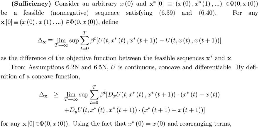
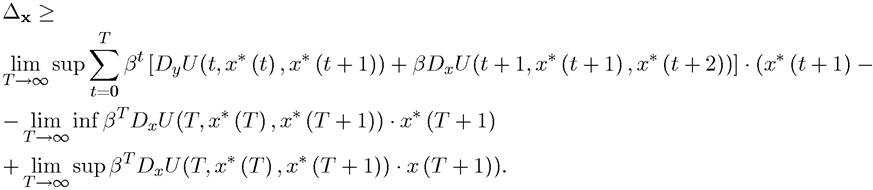
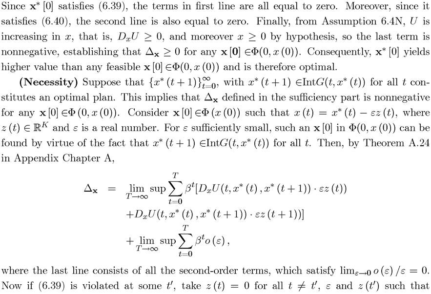
Proof of Theorem 6.12. The proof is very similar to that of Theorem 6.10.
x (t + 1))
6.7.3.
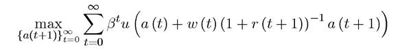
Application. As an application of nonstationary infinite-horizon optimization, let us consider the consumption problem in a market environment in which wages and interest rates are potentially changing over time.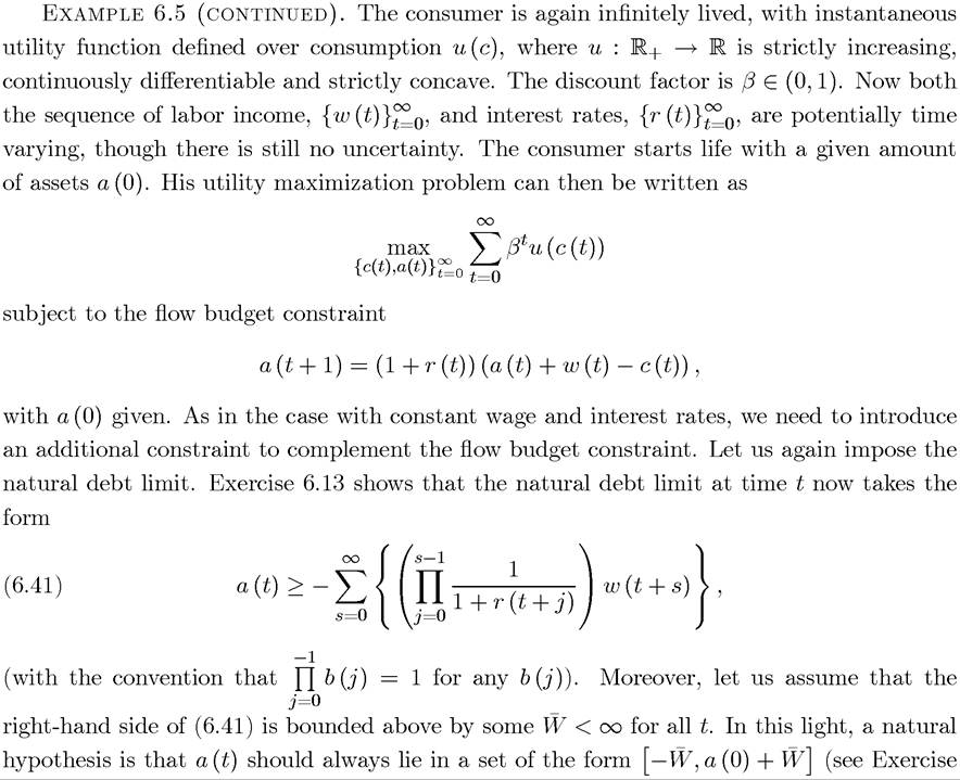
6.13). Repeating the same arguments as in Example 6.5, the consumer maximization problem can be written as
for given a (0). The Euler equation in this case is

for all t. Thus, instead of (6.37), we have the following more general consumption rule:
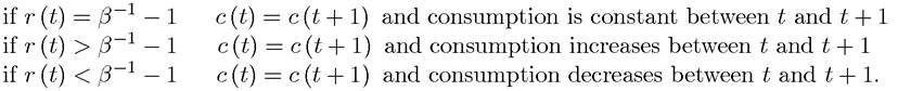
In some ways, this result is even more remarkable than the one in (6.37), since the “slope” of the optimal consumption path is not only independent of a (0), but it is also independent of current income and in fact of the entire sequence of income levels
6.8.