Fundamentals of Stationary Dynamic Programming
In this section, I return to the fundamentals of dynamic programming and show how they can be applied in a range of problems. The main result in this section is Theorem 6.10, which shows how dynamic first-order conditions, the Euler equations, together with the transversal- ity condition are sufficient to characterize solutions to dynamic optimization problems.
This theorem is arguably more useful in practice than the main dynamic programming theorems presented above.6.6.1. Basic Equations. Consider the functional equation corresponding to Problem
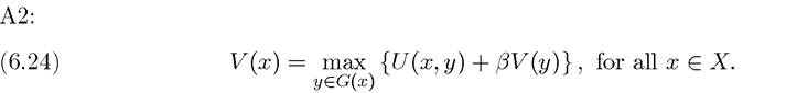
Let us assume throughout that Assumptions 6.1-6.5 hold. Then, from Theorem 6.4, the maximization problem in (6.24) is strictly concave, and from Theorem 6.6, the maximand is
224
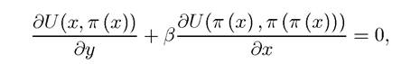
also differentiable. Therefore for any interior solution y ∈IntG (x), the first-order conditions are necessary and sufficient for an optimum (taking V (∙) as given). In particular, optimal solutions can be characterized by the following convenient Euler equations:

where I use *,s to denote optimal values and once again D denotes gradients (recall that, in the
The set of first-order conditions in eq. (6.25) would be sufficient to solve for the optimal policy, y*, if we knew the form of the V (∙) function. Since this function is determined recursively as part of the optimization problem, there is a little more work to do before we obtain the set of equations that can be solved for the optimal policy.
Fortunately, we can use the equivalent of the Envelope Theorem for dynamic programming (recall Theorem A.32 in Appendix Chapter A) and differentiate (6.24) with respect to the state vector, x, to obtain:
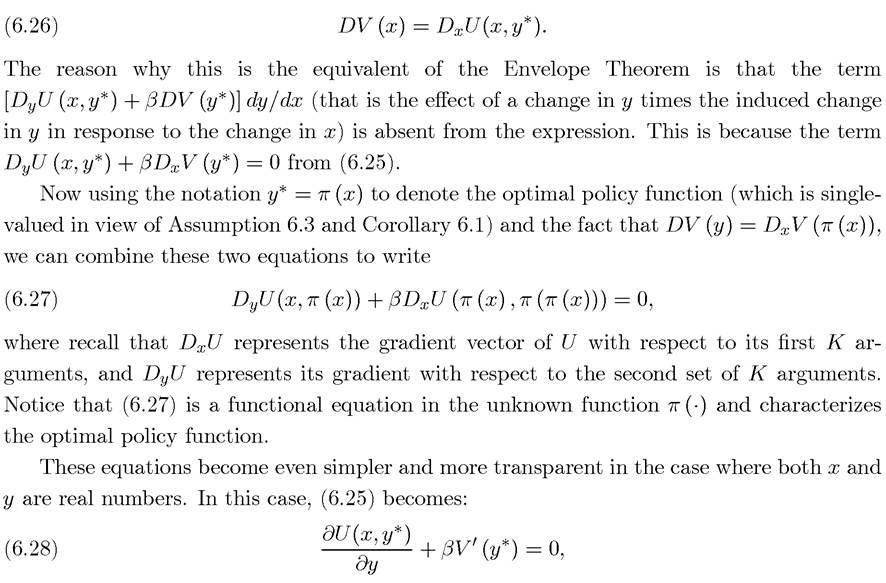
where V0 the notes the derivative of the V function with respect to its single argument.
This equation is very intuitive; it requires the sum of the marginal gain today from increasing y and the discounted marginal gain from increasing y on the value of all future returns to be equal to zero. For instance, as in Example 6.1, we can think of U as decreasing 225
in y and increasing in x; eq. (6.28) would then require the current cost of increasing y to be compensated by higher values tomorrow. In the context of growth, this corresponds to the current cost of reducing consumption to be compensated by higher consumption tomorrow. As with (6.25), the value of higher consumption in (6.28) is expressed in terms of the derivative of the value function, which is one of the unknowns. Let us now use the onedimensional version of (6.26) to find an expression for this derivative:
Now in this one-dimensional case, combining (6.29) together with (6.28) yields the following very simple condition:
where, in line with the notation for gradients, ∂U∕∂x denotes the derivative of U with respect to its first argument and ∂U∕∂y with respect to the second argument.
Alternatively, explicitly including the time arguments, the Euler equation can be written
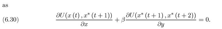
However, this Euler equation is not sufficient for optimality. In addition we need the transver- sality condition. The transversality condition is essential in infinite-dimensional problems, because it makes sure that there are no beneficial simultaneous changes in an infinite number of choice variables. In contrast, in finite-dimensional problems, there is no need for such a condition, since the first-order conditions are sufficient to rule out possible gains when we change many or all of the control variables at the same time.
The role that the transversal- ity condition plays in infinite-dimensional optimization problems will become more apparent after we see Theorem 6.10 and after the discussion in the next subsection.In the general case, the transversality condition takes the form:

where “•” denotes the inner product operator. In the one-dimensional case, we have the simpler transversality condition:
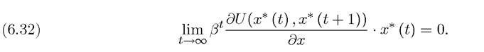
In words, this condition requires that the product of the marginal return from the state variable x times the value of this state variable does not increase asymptotically at a rate faster than or equal to 1∕β.
The next theorem shows that the transversality condition together with the transformed Euler equations in (6.27) are necessary and sufficient to characterize an optimal solution to Problem A1 and therefore to Problem A2.
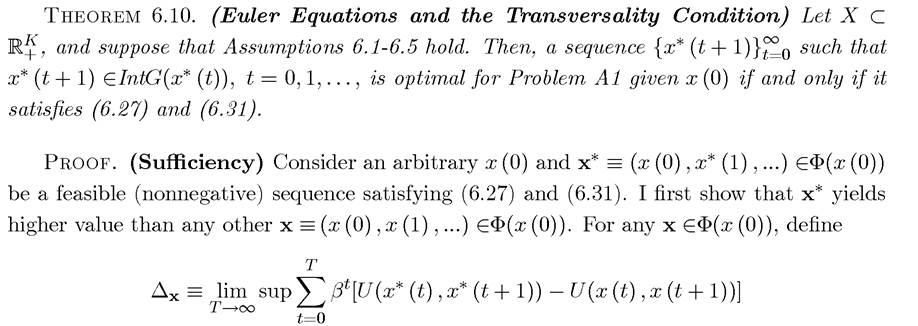
as the lim sup of the difference of the values of the objective function evaluated at the feasible sequences x* and x as the time horizon goes to infinity. Here lim sup is used instead of lim, since there is no guarantee that for an arbitrary x ∈Φ(x (0)), the limit exists.
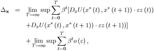
From Assumptions 6.2 and 6.5, U is continuous, concave, and differentiable. Since U is concave, Theorem A.24 and the multivariate equivalent of Corollary A.4 in Appendix Chapter A imply that
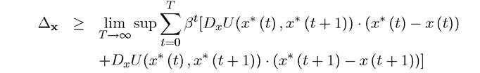
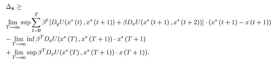
for any x ∈Φ(x (0)). Since x* (0) = x (0), DxU(x* (0),x* (1)) ∙ (x* (0) — x (0)) = 0. Therefore, we can rearrange terms in this expression to obtain
227
Chapter A,
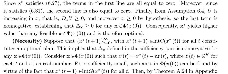
Theorem 6.10 shows that the simple form of the transversality condition, (6.31), is both necessary and sufficient sufficient for an interior optimal plan as long as the Euler equations, (6.27), are also satisfied.
The Euler equations, (6.27), are also necessary for an interior solution. Theorem 6.10 is therefore often all that we need to characterize solutions to dynamic optimization problems.I now illustrate how the tools that have been developed so far can be used in the context of the problem of optimal growth, which will be further discussed in Section 6.8.
EXAMPLE 6.4. Consider the following optimal growth, with log preferences, Cobb-Douglas technology and full depreciation of capital stock
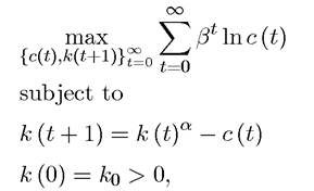

This is one of the canonical examples that admit an explicit-form characterization. To derive this characterization, let us follow Example 6.1 and set up the maximization problem in its recursive form as
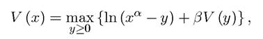
with x corresponding to today’s capital stock and y to tomorrow’s capital stock. Our main objective is to find the policy function y = π (x), which determines tomorrow’s capital stock as a function of today’s capital stock. Once this is done, we can easily determine the level of consumption as a function of today’s capital stock from the resource constraint.
It can be verified that this problem satisfies Assumptions 6.1-6.5. In particular, using the same argument as in Section 6.8, x and y again can be restricted to be in a compact set. Consequently, Theorems 6.1-6.6 apply. In particular, since V (∙) is differentiable, the Euler equation for the one-dimensional case, (6.28), implies
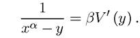
The Envelope condition, (6.29), gives:
V0 (x)
α — 1
αx
xα
- y
Thus using the notation y = π (x) and combining these two equations, we have
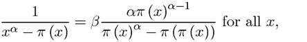
which is a functional equation in a single function, π (x).
There are no straightforward ways of solving functional equations, but in most cases guess-and-verify type methods are most fruitful. For example in this case, let us conjecture that
Substituting for this in the previous expression,
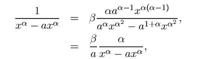
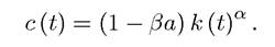
which implies that a = βα satisfies this equation. The policy function π (x) = βαxα also implies that the law of motion of the capital stock is

and the optimal consumption level is
It can then be verified that the capital-labor ratio k (t) converges to a steady state k*, which is sufficient to ensure the transversality condition (6.32). Corollary 6.1 and Theorem 6.10 then imply that π (x) = βαxα must be the unique policy function for this problem. Exercise 229
6.7 continues with some of the details of this example, and also shows how the optimal growth equilibrium involves a sequence of capital-labor ratios converging to a unique steady state.
Finally, let us have a brief look at the intertemporal utility maximization problem of a consumer facing a certain income sequence.
EXAMPLE 6.5. Consider the problem of an infinitely-lived consumer with instantaneous utility function defined over consumption u (c), where u is strictly increasing, contin
uously differentiable and strictly concave. The consumer discounts the future exponentially with the constant discount factor β ∈ (0,1). He also faces a certain (nonnegative) labor income stream of and starts life with a given amount of assets
 He receives
a constant net rate of interest r > 0 on his asset holdings (so that the gross rate of return is 1 + r). To start with, let us suppose that wages are constant, that is,
Then, the utility maximization problem of the consumer can be written as
subject to the flow budget constraint
a (t + 1) = (1+ r)(a (t) + w — c (t)),
with initial assets, a (0), given.
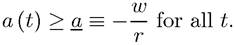
This maximization problem, without further constraints, is not well defined and in fact does not capture the utility maximization problem of the consumer. In particular, Exercise 6.11 shows that this problem allows the consumer to build up debt without limit (so that limt→∞ a (t) = -∞). This is sometimes referred to as a “Ponzi game” and involves the consumer continuously borrowing and rolling over debt. Moreover, clearly the consumer will prefer consumption paths that do this, since they enable him to increase his consumption at all dates. However, from an economic point of view this is a nonsensical solution and would not be feasible in a market economy, because the financial market (lenders) transacting with the consumer would make very large losses (at least asymptotically). This result emerges because we have not imposed the appropriate budget constraint on the consumer. As discussed in greater detail in Chapter 8, the flow budget constraint is not sufficient to capture the lifetime budget constraint of the consumer (and this is evidenced by the fact that the consumer can have consumption paths with limt→∞ a (t) = -∞). An additional constraint needs to be imposed so that the consumer cannot run such “Ponzi games”.There are three solutions to this problem. The first, which will be discussed in greater detail in Chapter 8 is to impose a “no-Ponzi condition” that rules out such schemes. The second is to assume that the consumer cannot borrow, so a (t) ≥ 0 for all t. While this prevents the problem, it is somewhat too “draconian”. For example, we may wish to allow the consumer to borrow temporarily, as many financial markets do, but not allow him to have an asset position reaching negative infinity. The third solution, which is in many ways the simplest, is to impose the natural debt limit. This essentially involves computing what
the maximum debt that the consumer can repay and then impose that his debt level should never fall below this. It is clear that, since consumption is nonnegative, the consumer can never repay more than his total wage income. Given a constant wage rate w and a constant interest rate r, the net present discounted value of the consumer’s wage income is w/r. This is a finite number, since w and r > 0. Therefore, if his asset holdings, a (t), ever fall below —w/r, the consumer will never be able to repay. It is therefore natural to expect the financial markets, even if they have the power to confiscate all of the income of the consumer, never to lend to such a level that a (t) < -w/ň for any t. In this light, the most economically natural additional constraint is to impose the natural debt limit and require that
id="Picutre 598" class="lazyload" data-src="/files/uch_group77/uch_pgroup317/uch_uch7365/image/image598.jpg">
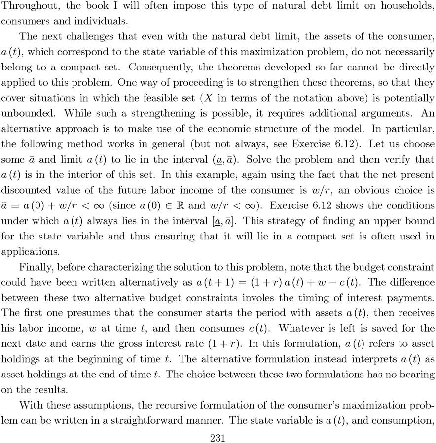
With standard arguments and denoting the current-value of the state variable by a and its future value by a0, the recursive form of this dynamic optimization problem can be written
as
This important equation is often referred to as the “consumption Euler” equation. It states that the marginal utility of current consumption must be equal to the marginal increase in the continuation value multiplied by the product of the discount factor, β, and the gross rate of return to savings, (1 + r). It captures the essential economic intuition of dynamic programming approach, which reduces the complex infinite-dimensional optimization problem to one of comparing today to “tomorrow”. As usual, the only difficulty here is that tomorrow itself will involve a complicated maximization problem and hence tomorrow’s value function and its derivative are endogenous. But here the Envelope condition, (6.29), again comes to our rescue and yields
where c0 refers to next period’s consumption. Using this relationship, the consumption Euler equation becomes

This form of the consumption Euler equation is more familiar and requires the marginal utility of consumption today to be equal to the marginal utility of consumption tomorrow multiplied
by the product of the discount factor and the gross rate of return. Since we have assumed that β and (1 + r) are constant, the relationship between today’s and tomorrow’s consumption never changes. In particular, since u (∙) is assumed to be continuously differentiable and strictly concave, u0 (∙) always exists and is strictly decreasing. Therefore, the intertemporal
consumption maximization problem implies the following simple rule:
(6.37)
The remarkable feature is that these statements have been made without any reference to the initial level of asset holdings a (0) and the wage rate w. It turns out that these only determine the initial level of consumption. The “slope” of the optimal consumption path is independent of the wealth of the individual. Exercise 6.13 asks you to determine the level of initial consumption using the transversality condition and the intertemporal budget constraint, while Exercise 6.12 asks you to verify that whenever r ≤ β — 1, a (t) ∈ (a, d) for all t (so that the artificial bounds on asset holdings that I imposed have no bearing on the results).
The example here is somewhat restrictive because wages are assumed to be constant over time. What happens if instead there is a time-varying sequence of wages What
What
happens if there is a time-varying sequence of interest rates Unfortunately, with a
time-varying sequence of wages or interest rates, the problem becomes nonstationary and the theorems developed for Problems A1 and A2 above no longer apply in this case. However, many equilibrium problems will have this feature, because individuals will be facing timevarying market prices. This motivates my discussion of nonstationary problems in the next section.
6.6.2. Dynamic Programming Versus the Sequence Problem. Before turning to nonstationary problems, let us compare the dynamic programming formulation to the sequence problem, and motivate the transversality condition using the sequence problem. Let us also suppose that x is one dimensional and that there is a finite horizon T. Then, the problem becomes
subject to x (t + 1) ≥ 0 with x (0) as given. Moreover, let U(x (T),x (T + 1)) be the last period’s utility, with x (T + 1) as the state variable left after the last period (this utility could be thought of as the “salvage value” for example).
In this case, we have a finite-dimensional optimization problem and we can simply look at first-order conditions. Moreover, let us again assume that the optimal solution lies in the interior of the constraint set, that is, x* (t) > 0, so that first-order conditions do not need to be expressed as complementary-slackness type conditions. In particular, in this case they take the following simple form, equivalent to the Euler equations above,

which are identical to the Euler equations for the infinite-horizon case (recall that ∂U∕∂x denotes the derivative of U with respect to its first argument and ∂U∕∂y with respect to the second argument). In addition, for x (T + 1), the following boundary condition is also necessary 
Intuitively, this boundary condition requires that x* (T + 1) should be positive only if an interior value of it maximizes the salvage value at the end. To provide more intuition for this expression, let us return to the formulation of the optimal growth problem in Example 6.1.
EXAMPLE 6.6. Recall that in terms of the optimal growth problem,

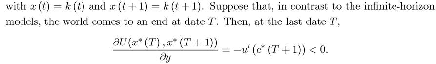
From (6.38) and the fact that U is increasing in its first argument (Assumption 6.4), an optimal path must have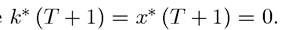 Intuitively, there should be no capital
left at the end of the world. If any resources were left after the end of the world, utility could be improved by consuming them either at the last date or at some earlier date.
Now, the transversality condition can be derived heuristically as an extension of condition (6.38) to the case where T = ∞. Taking this limit,
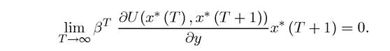
Moreover, as T → ∞, the Euler equation implies
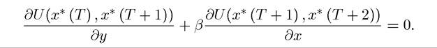
Substituting this relationship into the previous equation,
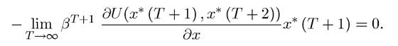
Canceling the negative sign, and changing the timing for convenience:
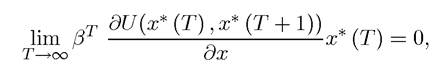
which is exactly the transversality condition in (6.32). This derivation also highlights that the transversality condition can equivalently be written as
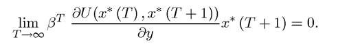
This emphasizes that there is no unique representation of the transversality condition, but various different equivalent forms. They all correspond to a “boundary condition at infinity” ruling out variations that change an infinite number of control variables at the same time.
234
6.7.