Proofs of the Main Dynamic Programming Theorems*
I now provide proofs of Theorems 6.1-6.6. The first step is a straightforward lemma, which will be useful in these proofs. For a feasible infinite sequence x = (x (0) ,χ (1),...) ∈Φ(x (0)) starting at x (0), let
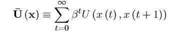
be the value of choosing this potentially non-optimal infinite feasible sequence.
In view of Assumption 6.1, exists and is finite. The next lemma shows that
 ) can be separated into two parts, the current return and the continuation return.
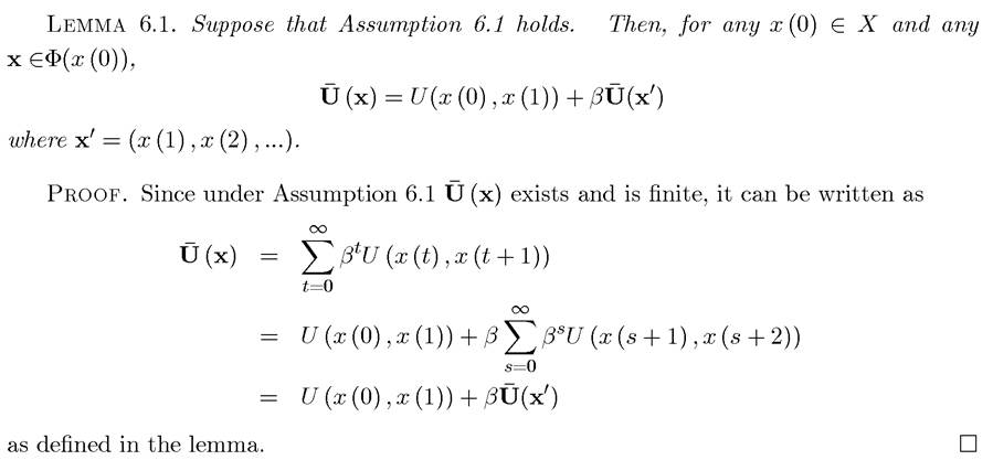
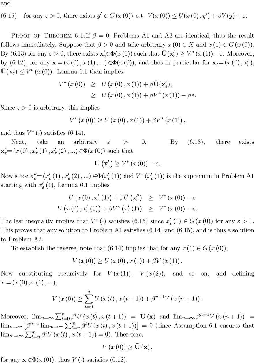
Before providing a proof of Theorem 6.1, it is useful to be more explicit about what it means for V and V * to be solutions to Problems A1 and A2. Let us start with Problem A1. Using the notation introduced in this section, for any x (0) ∈ X,
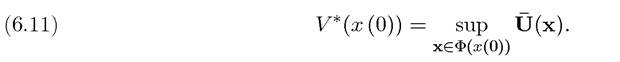
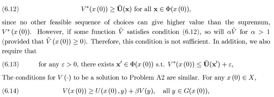
In view of Assumption 6.1, which ensures that all values are bounded, (6.11) implies
217
In economic problems, we are often interested not in the maximal value of the program but in the optimal plans that achieve this maximal value. Recall that the question of whether the optimal path resulting from Problems A1 and A2 are equivalent was addressed by Theorem
6.2.
I now provide a proof of this theorem.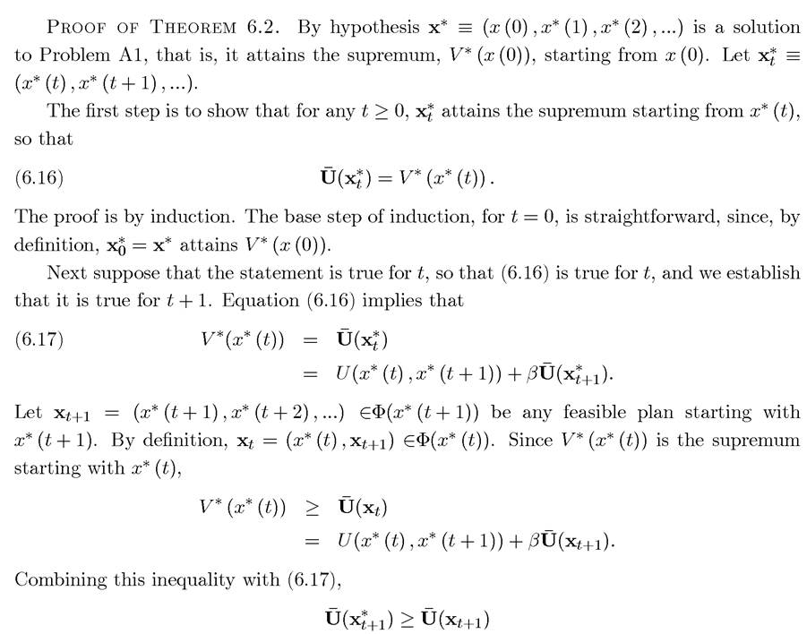
219
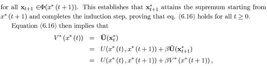
establishing (6.3) and thus completing the proof of the first part of the theorem.
Now suppose that (6.3) holds for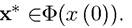 Then, substituting repeatedly for x*,
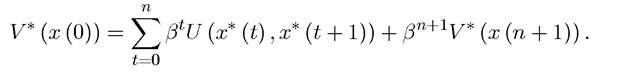
In view of the fact that V * (∙) is bounded (cf. Assumption 6.1),
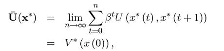
thus x* attains the optimal value in Problem A1, completing the proof of the second part of the theorem. ?
These two theorems establish that under Assumptions 6.1 and 6.2, we can freely interchange Problems A1 and A2. Our next task is to prove that a policy achieving the optimal path exists for both problems. I will provide two alternative proofs for this to show how this conclusion can be reached either by looking at Problem A1 or at Problem A2, and then exploiting their equivalence. The first proof is more abstract and works directly on the sequence problem, Problem A1. This method of proof will be particularly useful when we look at nonstationary problems. 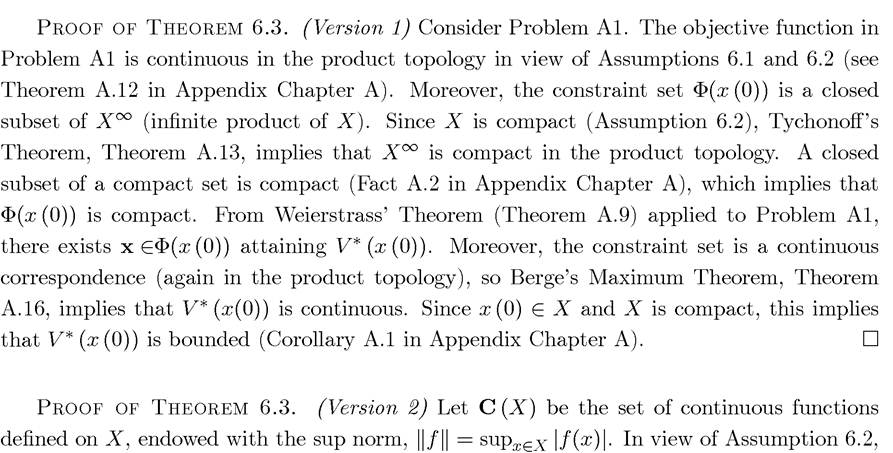
the relevant set X is compact and therefore all functions in C (X) are bounded since they are continuous and X is compact (Corollary A.1 in Chapter A). For V ∈ C (X), define the operator T as

A fixed point of this operator, V = TV, will be a solution to Problem A2. We first prove that such a fixed point (solution) exists. The maximization problem on the right-hand side of (6.18) is one of maximizing a continuous function over a compact set, and by Weierstrass’s Theorem, Theorem A.9, it has a solution.
Consequently, T is well-defined. Moreover, because G (x) is a nonempty and continuous correspondence by Assumption 6.1, and U (x, y^) and V (y) are continuous by hypothesis, Berge’s Maximum Theorem, Theorem A.16, implies that
is continuous in x, thus TV (x) ∈ C (X) and T maps C (X) into itself.
Next, it is also straightforward to verify that T satisfies Blackwell’s sufficient conditions for a contraction in Theorem 6.9 (see Exercise 6.6). Therefore, applying Theorem 6.7, a unique fixed point V ∈ C(X) to (6.18) exists and this is also the unique solution to Problem A2.
Now consider the maximization in Problem A2. Since U and V are continuous and G (x) is compact-valued, another application of Weierstrass’s Theorem implies that y ∈ G (x) achieving the maximum exists. This defines the set of maximizers Π (x) for Problem A2, that is,
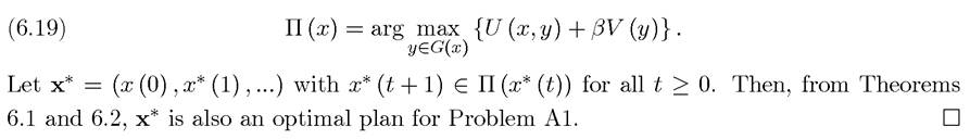
An additional result that follows from the second version of the theorem (which can also be derived from version 1, but would require more work), concerns the properties of the set of maximizers Π (x) (or equivalently the correspondence defined in (6.19). An
immediate application of the Berge’s Maximum Theorem, Theorem A.16, implies that Π is a upper hemi-continuous and compact-valued correspondence. This observation will be used in the proof of Corollary 6.1. Before turning to this corollary, I provide a proof of Theorem
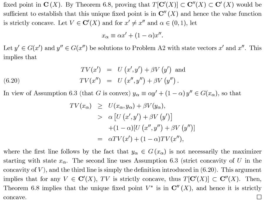
6.4. This proof also shows how the Contraction Mapping Theorem, Theorem 6.8, is often used in the study of dynamic optimization problems.
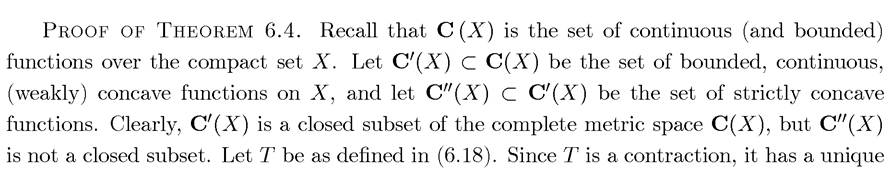
221
proof OF Corollary 6.1.
Assumption 6.3 implies that U (x,y) is concave in y, and under this assumption, Theorem 6.4 established that V (y) is strictly concave in y. The sum of a concave function and a strictly concave function is strictly concave, thus the right-hand side of Problem A2 is strictly concave in y. Therefore, combined with the fact that G (x) is convex for each x ∈ X (again Assumption 6.3), there exists a unique maximizer y ∈ G (x) for each x ∈ X. This implies that the policy correspondence Π (x) is single-valued, thus a function, and can thus be expressed as π (x). Since Π (x) is upper hemi-continuous as observed above, so is π(x). Since a single-valued upper hemi-continuous correspondence is a continuous function, the corollary follows.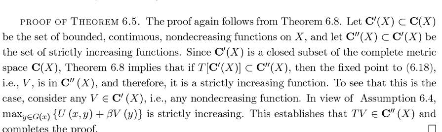 ?
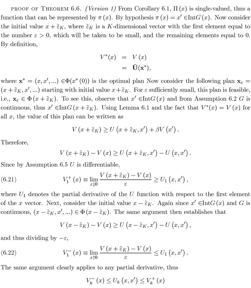
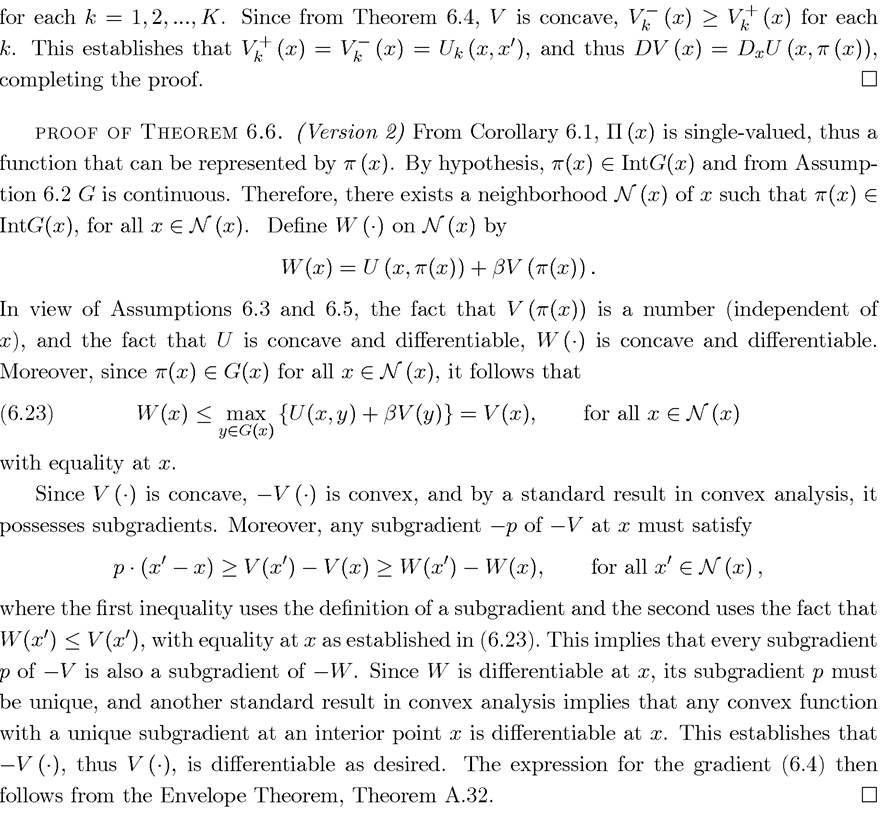
? For Theorem 6.6, I also provide two proofs. The first one is simpler and only establishes that V (x^) has a well-defined matrix of partial derivatives, the Jacobian, DV (x). The second proof appeals to a powerful result from convex analysis and establishes that V (x) is differentiable (see Appendix Chapter A for examples of functions that may possess well-defined Jacobians but may not be differentiable). Moreover, the second proof is more widely known and used in the literature. For this proof, recall that ε ∣ 0 implies that ε is a positive decreasing sequence approaching 0 and that ε is a negative increasing sequence approaching 0.
6.6.