Discrete-Time Infinite-Horizon Optimization
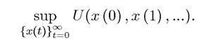
The canonical discrete-time infinite-horizon optimization program can be written as 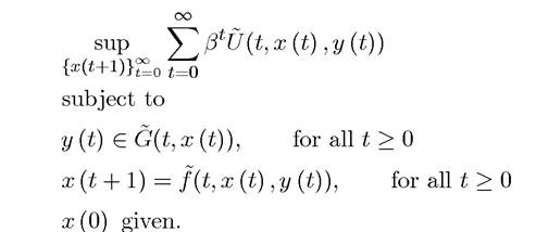
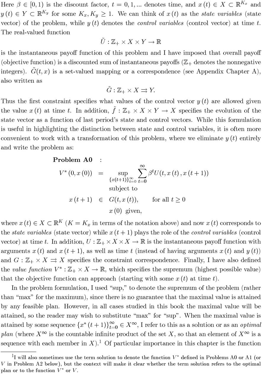
V * (t,x), which can be thought of as the value function, meaning the value of pursuing the optimal strategy starting with initial state x at time t.
Our objective is to characterize the optimal plan and the value function
A more general formulation would involve undiscounted ob jective function, written as
This added generality is not particularly useful for most of problems in economic growth and the discounted objective function ensures time-consistency as discussed in Exercise 5.1, in the sense that at a later date the decision maker will have no reason to revise the optimal plan she chooses at time t = O.
Problem A0 is somewhat abstract. However, it has the advantage of being tractable and general enough to nest many interesting economic applications. The next example shows how the canonical optimal growth problem can be put into this language.
EXAMPLE 6.1. Recall the optimal growth problem introduced in Section 5.9 of the previous chapter,
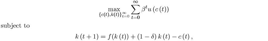
k (t) ≥ 0 and given k (0) > 0, with u : This problem maps into the general
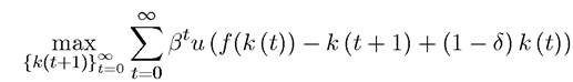
formulation here with a simple one-dimensional state and control variables. In particular, let x (t) = k (t) and x (t + 1) = k (t + 1). Then, use the constraint to write:
c (t) — f (k (t)) — k (t + 1) + (1 — δ) k (t),
and substitute this into the objective function to obtain:

A notable feature emphasized by Example 6.1 is that once the optimal growth problem is formulated in the language of Problem A0, U and G do not explicitly depend on time. This is a fairly common feature. Many interesting problems in economics can be formulated in a stationary form, meaning that the objective function is a discounted sum, and U and G do not explicitly depend on time. In the next section, I start with the study of stationary dynamic optimization problems, returning to the more general case of Problem A0 in Section 6.7.
205
6.2.