Infinite-Horizon Optimal Control
The results presented so far are most useful in developing an intuition for how dynamic optimization in continuous time works. While a number of problems in economics require finite- horizon optimal control, most economic problems—including almost all growth models—are more naturally formulated as infinite-horizon problems.
This is obvious in the context of economic growth, but is also the case in repeated games, political economy or industrial organization, where even if individuals may have finite expected lives, the end date of the game or of their lives may be uncertain. For this reason, the canonical model of optimization in economic problems is the infinite-horizon one. In this section, I provide necessary and sufficient conditions for optimality in infinite-horizon optimal control problems. Since these are the results that are most often used in economic applications, I simplify the exposition 267and state these results for the case in which both the state variable and the control variable are one dimensional. The more general, multivariate case is discussed in Section 7.6, when I return to the issues of existence of solutions and properties of the value functions.
7.3.1. The Basic Problem: Necessary and Sufficient Conditions. Let us focus on infinite-horizon control with a single control and a single state variable. For reasons that will be explained below, it is useful to generalize the terminal value constraint on the state variable. For this purpose, throughout this chapter, such that
exists and satisfies Then, the terminal value condition on the state variable will be specified as
 for some
 The special case where
b (t) = 1 gives us the terminal value constraint as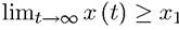 and is sufficient in many
applications.
But for the analysis of competitive equilibrium in continuous time, we will need a terminal value constraint of the form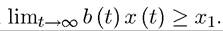 Now using the same notation
 as above, the infinite-horizon optimal control problem is
and


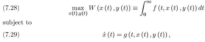
The main difference is that now time runs to infinity. Note also that this problem allows for an implicit choice over the endpoint xχ, since there is no terminal date. The last part of (7.30) imposes a lower bound on this endpoint. In addition, I have further simplified the problem by removing the feasibility requirement that the control y (t) should always belong to the set Y (t) and that x (t) should belong to the set X (t), instead simply requiring both to be real-valued functions of time. Because the state variable x (t) does not necessarily lie in a compact set, the results developed here can be applied to endogenous growth models.
The definition of an admissible pair (x (t),y (t)) is defined in the same way as above (in particular, recall footnote 1). Since x (t) is given by a continuous differential equation, when y (t) is continuous, x (t) will be differentiable and when y (t) is piecewise continuous (meaning that it has a finite number of jumps), x (t) will be differentiable almost everywhere.
There are a number of technical difficulties when dealing with the infinite-horizon case, which are similar to those in the discrete-time analysis. Primary among those is the fact that the value of the functional in (7.28) may not be finite. These issues will be dealt with below.
The main theorem for the infinite-horizon optimal control problem is the following more general version of the Maximum Principle.
Before stating this theorem, let us recall that the Hamiltonian is defined by (7.12), with the only difference that the horizon is now infinite.In addition, let us define the value function, which is the analog of the value function in discrete-time dynamic programming introduced in the previous chapter:
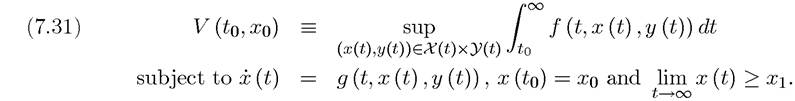
In words, V (to,xo) gives the optimal value of the dynamic maximization problem starting at time to with state variable xo. Clearly,

Our first result is a weaker version of the Principle of Optimality, which we encountered in the context of discrete-time dynamic programming in the previous chapter:
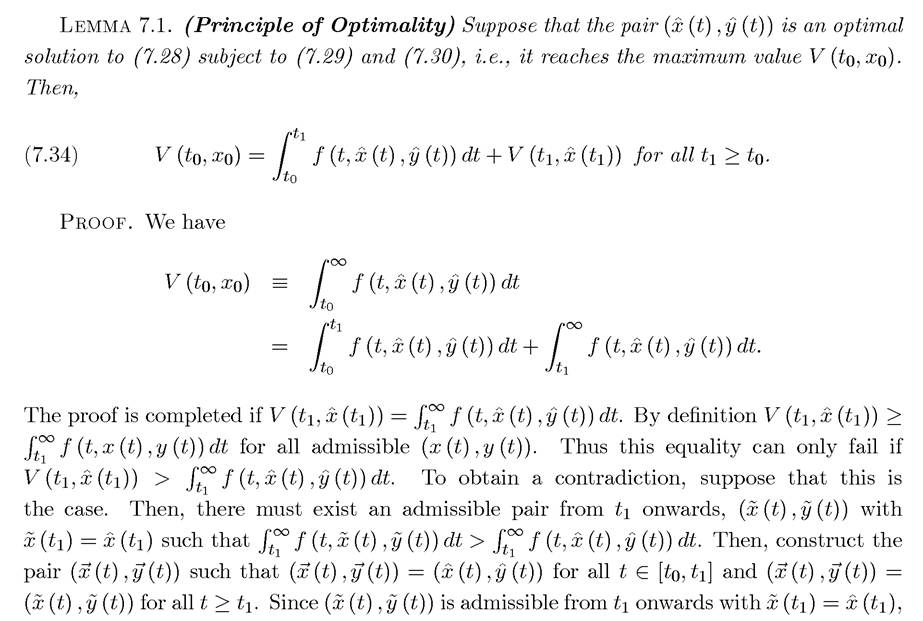
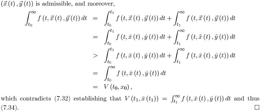
Two features in this version of the Principle of Optimality are noteworthy. First, in contrast to the similar equation in the previous chapter, it may appear that there is no discounting in (7.34). This is not the case, since the discounting is embedded in the instantaneous payoff function f, and is thus implicit in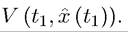 Second, this lemma may appear
to contradict the discussion of “time-consistency” in the previous chapter, since the lemma is stated without additional assumptions that ensure time-consistency. The important point here is that in the time-consistency discussion, the decision-maker considered updating his or her plan, with the payoff function being potentially different after date tι (at least because bygones were bygones). In contrast, here the payoff function remains constant.
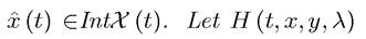
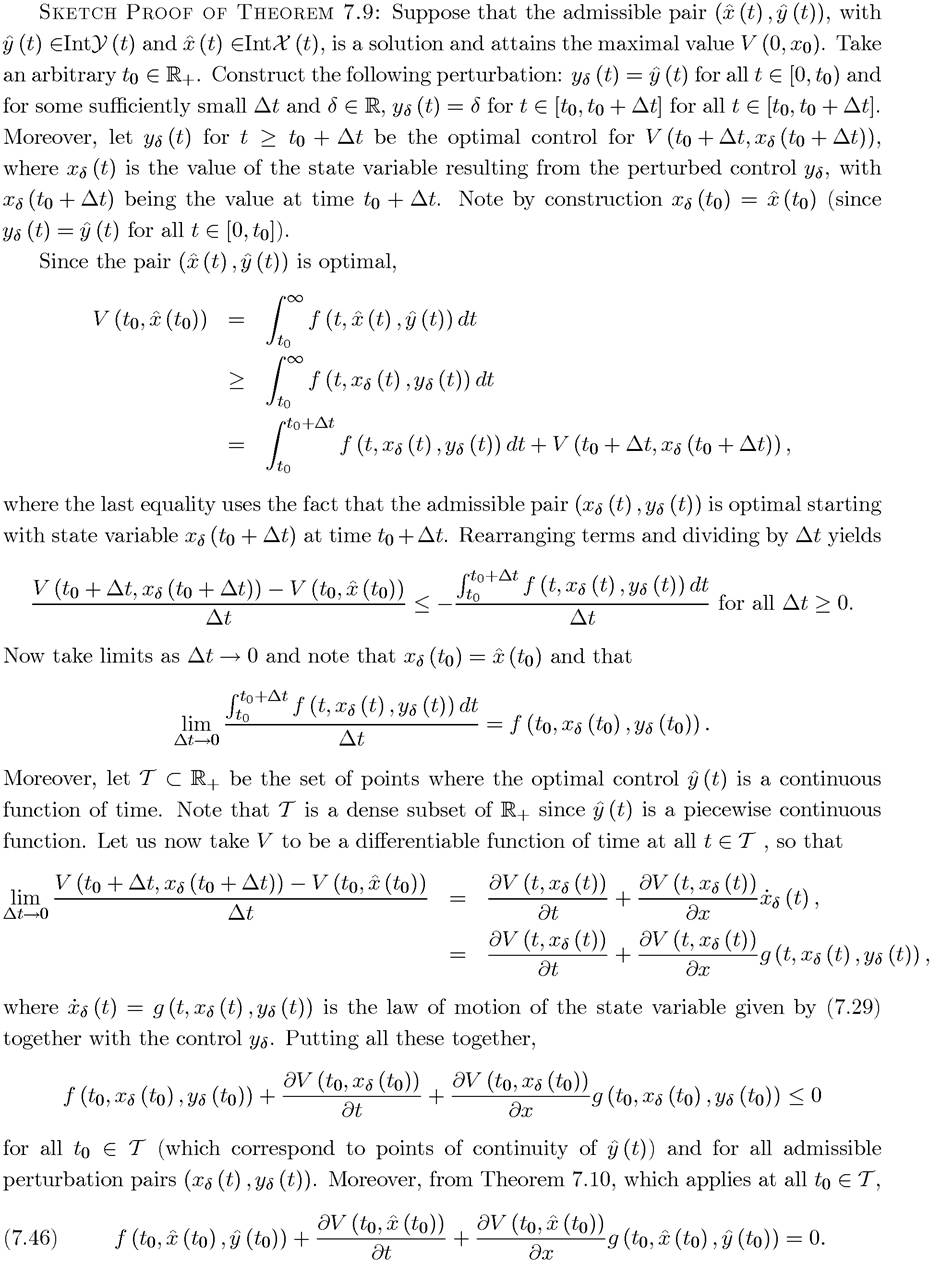
The issue of time-consistency is discussed further in Exercise 7.22. I next state one of the main results on necessary conditions. In this theorem, I also slightly relax the assumption that the optimal control y (t) is continuous.Theorem 7.9. (Infinite-Horizon Maximum Principle) Suppose that problem of maximizing (7.28) subject to (7.29) and (7.30), with f and g continuously differentiable, has a piecewise continuous interior solution,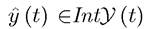 with a corresponding state variable
 be defined in (7.12). Then, the optimal control
 and the corresponding path of the state variable
 are such that the Hamiltonian H (t, x, y, λ) satisfies the Maximum Principle, that

for all y (t) ∈ Y (t) and for all t ∈ R. Moreover, whenever y (t) is continuous, the following necessary conditions are satisfied: 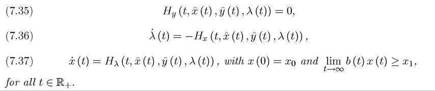
The proof of this theorem is relatively long and will be provided later in this section. Notice that whenever an optimal solution of the specified form exists, it satisfies the Maximum Principle. Thus in some ways Theorem 7.9 can be viewed as stronger than the theorems presented in the previous chapter, especially since it does not impose compactness type conditions. Nevertheless, this theorem only applies when the maximization problem has a piecewise continuous solution y (t).[13] In addition, Theorem 7.9 states that if the optimal control, y (t), is a continuous function of time, conditions (7.35)-(7.37) are satisfied everywhere.
The fact that y (t) is a piecewise continuous function implies that the optimal control may include discontinuities, but these will be relatively “rare”—in particular, it will be continuous “most of the time”. The added generality of allowing discontinuities is somewhat superfluous in most economic applications, because economic problems often have enough structure to ensure that y (t) is indeed a continuous function of time. Consequently, in most economic problems (and in all of the models studied in this book) it will be sufficient to focus on the necessary conditions (7.35)-(7.37).It is also useful to have a different version of the necessary conditions in Theorem 7.9, which are directly comparable to the necessary conditions generated by dynamic programming in the discrete-time dynamic optimization problems studied in the previous chapter. In particular, the necessary conditions can also be expressed in the form of the so-called Hamilton-Jacobi-Bellman (HJB) equation.
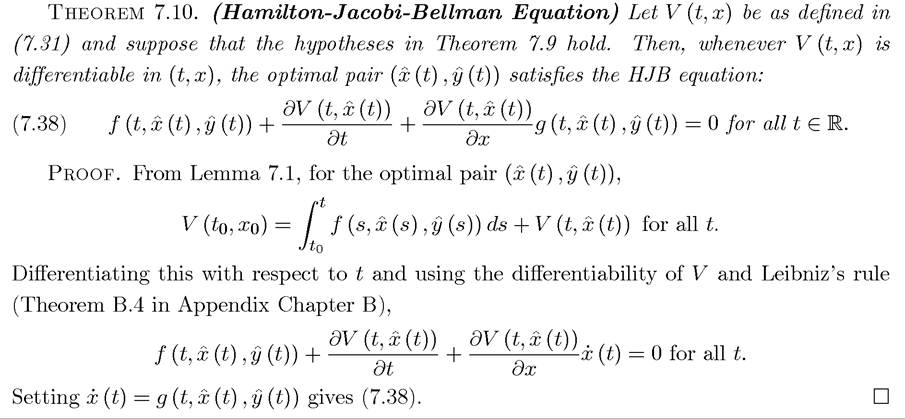
The HJB equation will be useful in providing an intuition for the Maximum Principle. More importantly, it is used directly in many economic models, including in the endogenous technology models studied in Part 4 below.
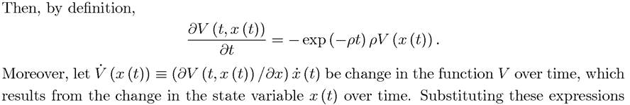
It is also worth noting a few important features concerning the HJB equation. First, given that the continuous differentiability of f and g, the assumption that V (t, x) is differentiable is not very restrictive, though it is not always satisfied. From the definition (7.31), at all t where  ł is continuous and g (t,x,y^) is differentiable in t, V (t, x) will also be differentiable in t. Moreover, an Envelope Theorem type argument also implies that when
 is continuous, V (t, x) should also be differentiable in x (the differentiability of V (t, x) in x can also be established directly, see Theorem 7.17 below). Second, (7.38) is a partial differential equation, since it features the derivative of V with respect to both time and the state variable x.
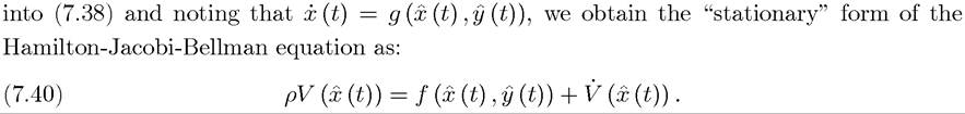
7.3.2. Heuristic Derivation of the Stationary HJB Equation. Given its prominent role in dynamic economic analysis, it is useful to provide an alternative heuristic (and more “intuitive”) proof of the HJB equation. For this purpose, let us focus on the simpler stationary version of the HJB equation. This stationary version applies to exponentially discounted maximization problems with time-autonomous constraints (see Sections 7.5 and 7.7 below). Briefly, in these problems the payoff function is exponentially discounted, that is,

and the law of motion of the state variable is given by an autonomous differential equation, that is,
In this case, one can easily verify that if an admissible pair is optimal starting
at t = 0 with initial condition x (0) = xo, then it is also optimal starting at s > 0, starting with the same initial condition, that is, is optimal for the problem with initial
condition x (s) = xo (see Exercise 7.16). In view of this, let us define V (x) ? V (0,x), that is, the value of pursuing the optimal plan ι starting with initial condition x, evaluated
at t = 0. Since is an optimal plan regardless of the starting date,
(7.39) V (t, x (t)) ? exp (—pt) V (x (t)).
This stationary HJB equation is widely used in dynamic economic analysis and can be interpreted as a “no-arbitrage asset value equation,” as discussed in subsection 7.3.4 below. The following heuristic argument not only shows how this equation is derived, but also provides a further intuition.
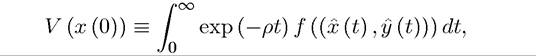
Heuristic Derivation of the Stationary HJB Equation (7.40): Consider the discounted infinite-horizon problem described above and suppose that the admissible pair (x (t), y(t)) is optimal starting at t = 0 with initial condition x (0). Recall that the value function starting at x (0) is defined as
exp (—pt) at t = 0. Substituting these terms into (7.41),

Rearranging, this is identical to (7.40). ?
7.3.3. Transversality Condition and Sufficiency. Since there is no terminal value
constraint of the form in Theorem 7.9, we may therefore may expect that there
should be a transversality condition similar to the condition that λ (tι) = 0 in Theorem 7.1. For example, we may be tempted to impose a transversality condition of the form

which would be generalizing the condition that λ (tι) = 0 in Theorem 7.1. But this is not in general the case. A milder transversality condition of the form

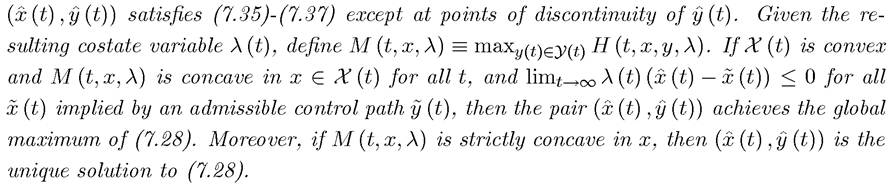
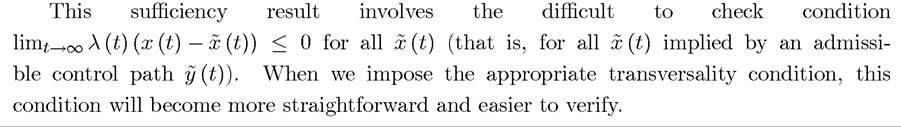
for an admissible pair (x (t), y(t^)^) satisfying the necessary conditions applies under relatively mild conditions (see Theorem 7.12 below), but is not easy to check. Stronger transversality conditions apply when we put more structure on the problem (see Section 7.4 below). Before presenting these results, there are immediate generalizations of the sufficiency theorems to this case.
Theorem 7.11. (Sufficiency Conditions for Infinite-Horizon Optimal Control) Consider the problem of maximizing (7.28) subject to (7.29) and (7.30), with f and g continuously differentiable. Define H (t,x,y,λ) as in (7.12), and suppose that an admissible pair
Proof. See Exercise 7.13. ?
7.3.4. Economic Intuition. The Maximum Principle is not only a powerful mathematical tool, but from an economic point of view, it is the right tool, because it captures the essential economic intuition of dynamic economic problems. In this subsection, we provide two different and complementary economic intuitions for the Maximum Principle. One of them is based on the original form as stated in Theorem 7.4 or Theorem 7.9, while the other is based on the dynamic programming (HJB) version provided in Theorem 7.10.
7
'Here I am using the language of “relaxing the constraint” implicitly presuming that a high value of x (t) contributes to increasing the value of the objective function. This simplifies terminology, but it is not necessary for any of the arguments, since λ (t) can be negative.
The second and complementary intuition for the Maximum Principle comes from the HJB equation (7.38) in Theorem 7.10. In particular, let us consider the exponentially discounted problem discussed above (and in greater detail in Section 7.5 below). Recall that in this case, the “stationary” form of the Hamilton-Jacobi-Bellman equation takes

This widely-used equation can be interpreted as a “no-arbitrage asset value equation”. Intuitively, we can think of V as the value of an asset traded in the stock market and ρ as the required rate of return for (a large number of) investors. When will investors be happy to hold this asset? Loosely speaking, they will do so when the asset pays out at least the required rate of return. In contrast, if the asset pays out more than the required rate of return, there would be excess demand for it from the investors until its value adjusts so that its rate of return becomes equal to the “required rate of return”. Therefore, we can think of the return on this asset in “equilibrium” being equal to the required rate of return, ρ. The return on the assets come from two sources: first, “dividends,” that is, current returns paid out to investors. In the current context, this corresponds to the flow payoff
If this dividend were constant and equal to d, and there were no other returns, then the no-arbitrage condition would imply V = d/p or
pV = d.
However, in general the returns to the holding an asset come not only from dividends but also from capital gains or losses (appreciation or depreciation of the asset). In the current context, this is equal to V. Therefore, instead of pV = d, the no-arbitrage condition becomes
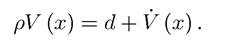
Thus, at an intuitive level, the Maximum Principle (for stationary problems) amounts to requiring that the maximized value of dynamic maximization program, V (x), and its rate of change, IJ (x), should be consistent with this no-arbitrage condition.
7.3.5. Proof of Theorem 7.9*. In this subsection, I provide a sketch of the proof of Theorem 7.9. A fully rigorous proof of Theorem 7.9 is quite long and involved. It can be found in a number of sources mentioned in the references below. The version provided here contains all the basic ideas, but is stated under the assumption that V (t, x^) is twice differentiable in t and x. As discussed above, the assumption that V (t, x) is differentiable in t and x is not particularly restrictive and Theorem 7.17 below provide sufficient conditions for this to be the case. Nevertheless, the additional assumption that it is twice differentiable is somewhat more stringent.
The main idea of the proof is due to Pontryagin and co-authors. Instead of smooth variations from the optimal pair the method of proof considers “needle-like”
variations, that is, piecewise continuous paths for the control variable that can deviate from the optimal control path by an arbitrary amount for a small interval of time.
7.4.