More on Transversality Conditions

I next turn to a study of the boundary conditions at infinity in infinite-horizon maximiza­tion problems. As in the discrete-time optimization problems, these limiting boundary condi­tions are referred to as “transversality conditions”.

following example, which is very close to the original model that Frank Ramsey studied in 1928, illustrates that this is not the case; without further assumptions, the valid transversality condition is given by the weaker condition (7.43).

Example 7.2. Consider the following problem:

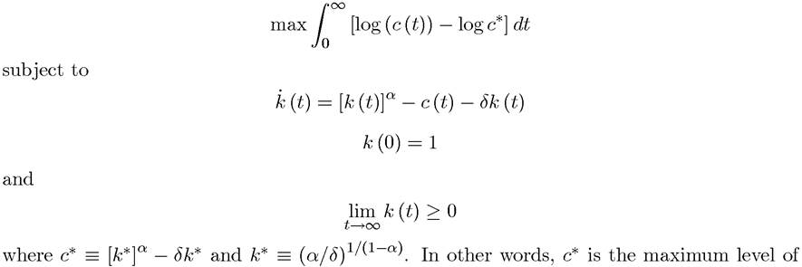
consumption that can be achieved in the steady state of this model and k* is the corresponding steady-state level of capital. This way of writing the objective function makes sure that the integral converges and takes a finite value (since c (t) cannot exceed c* forever).

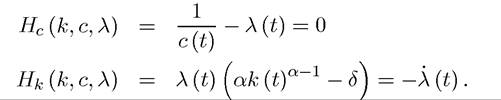
The Hamiltonian is straightforward to construct; it does not explicitly depend on time and takes the form

and implies the following necessary conditions

It can be verified that any optimal path must feature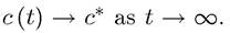This, however,

implies that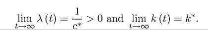

Now recall from Theorem 7.3 that the finite-horizon transversality condition in this case would have beenTherefore,

the equivalent of th finite-horizon transversality conditions do not hold.

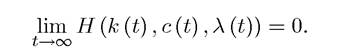
The next theorem shows that this is indeed a useful transversality condition for infinite­horizon optimization problems.

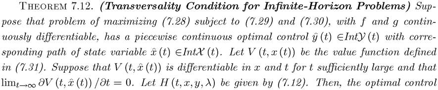
y (t) and the corresponding path of the state variable x (t) satisfy the necessary conditions (7.35)-(7.37) and the transversality condition

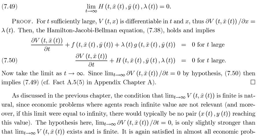
lems and will be satisfied in all of the models studied in this book. However, the transversality condition (7.49) is not particularly convenient to work with. In the next section, I present a stronger and more useful version of this transversality condition that applies in the context of discounted infinite-horizon problems.

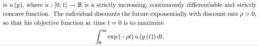
EXAMPLE 7.3. One of the most common examples of this type of dynamic optimization prob­lem is that of the optimal time path of consuming a non-renewable resource. In particular, imagine the problem of an infinitely-lived individual that has access to a non-renewable or exhaustible resource of size 1. The instantaneous utility of consuming a flow of resources y

The constraint is that the remaining size of the resource at time t, x (t) evolves according to 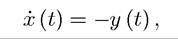which captures the fact that the resource is not renewable and becomes depleted as more of it is consumed. Naturally, we also need that x (t) ≥ 0.

The current-value Hamiltonian takes the form

Theorem 7.13 implies the following necessary condition for an interior continuously differen­tiable solutionto this problem.

and

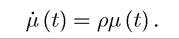
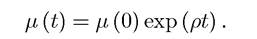
The second condition follows since neither the constraint nor the objective function depend on x (t). This is the famous Hotelling rule for the exploitation of exhaustible resources. It charts a path for the shadow value of the exhaustible resource. In particular, integrating both sides of this equation we obtain

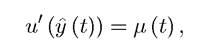
Now combining this with the first-order condition for y (t),

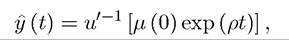
where_{l j} is the inverse function of u', which exists and is strictly decreasing by virtue of the fact that u is strictly concave. This equation immediately implies that the amount of the resource consumed is monotonically decreasing over time. This is economically intuitive: because of discounting, there is preference for early consumption, whereas delayed consump­tion has no return (there is no production or interest payments on the stock). Nevertheless, the entire resource is not consumed immediately, since there is also a preference for smooth consumption arising from the fact that u (∙) is strictly concave.

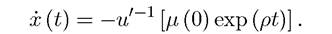
Combining the previous equation with the resource constraint gives

Integrating this equation and using the terminal value constraint that x (0) = 1,

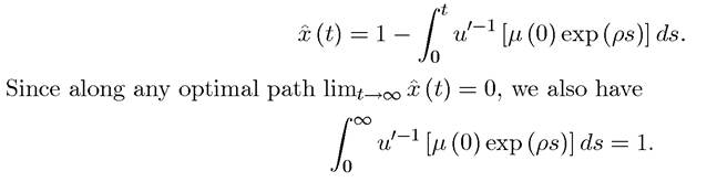
Therefore, the initial value of the costate variable μ (0) must be chosen so as to satisfy this equation. You are asked to verify that the transversality condition (7.49) is satisfied in Exercise 7.19.

7.5.