Discounted Infinite-Horizon Optimal Control
Part of the difficulty, especially regarding the absence of a transversality condition, comes from the fact that we did not impose enough structure on the functions f and g. As discussed above, our interest is with the growth models where the utility is discounted exponentially.
Consequently, economically interesting problems often take the following more specific form:
subject to

and

where recall again that b :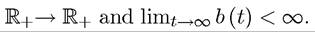 Throughout the assumption that
there is in fact discounting, that is, p > 0, is implicit.
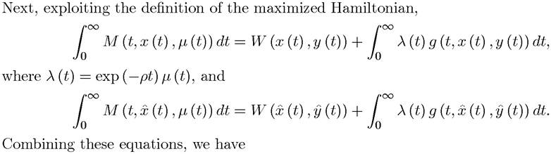
The special feature of this problem is that the objective function, f, depends on time only through exponential discounting. The Hamiltonian in this case would be: 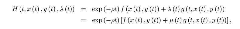 where the second line defines

In fact, in this case, rather than working with the standard Hamiltonian, we can work with the current-value Hamiltonian, defined as

When g (t, x (t),y (t)) is also an autonomous differential equation of the form g (x (t),y (t)), I simplify the notation by writing
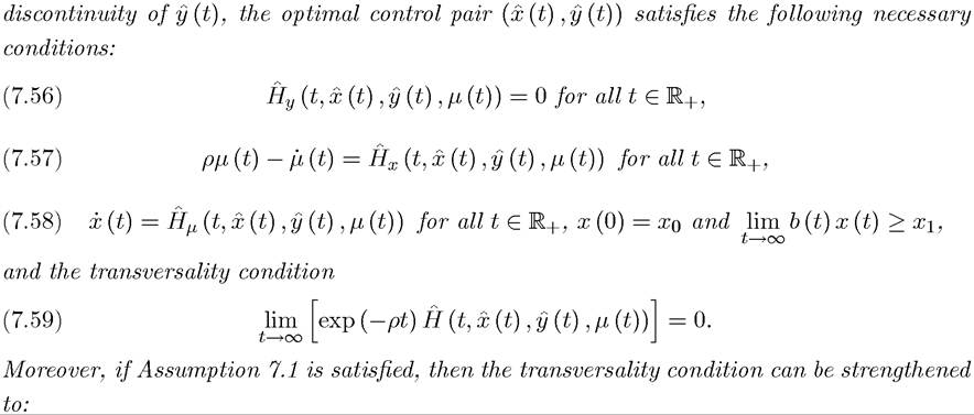
The next result establishes the necessity of a stronger transversality condition under some additional assumptions. These assumptions can be relaxed, though the result is simpler to understand and prove under these assumptions, and they are typically met in economic applications.
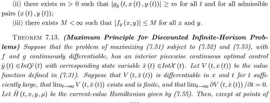
Throughout, f and g are continuously differentiable for all admissible (x (t),y (t)) (with derivatives fx, fy, gx and gy).Assumption 7.1: In the maximization of (7.51) subject to (7.52) and (7.53):
(i) f is weakly monotone in (x,y) and g is weakly monotone in (t,x,y) (for example, f could be nondecreasing in x and nonincreasing in y, and so on);
282
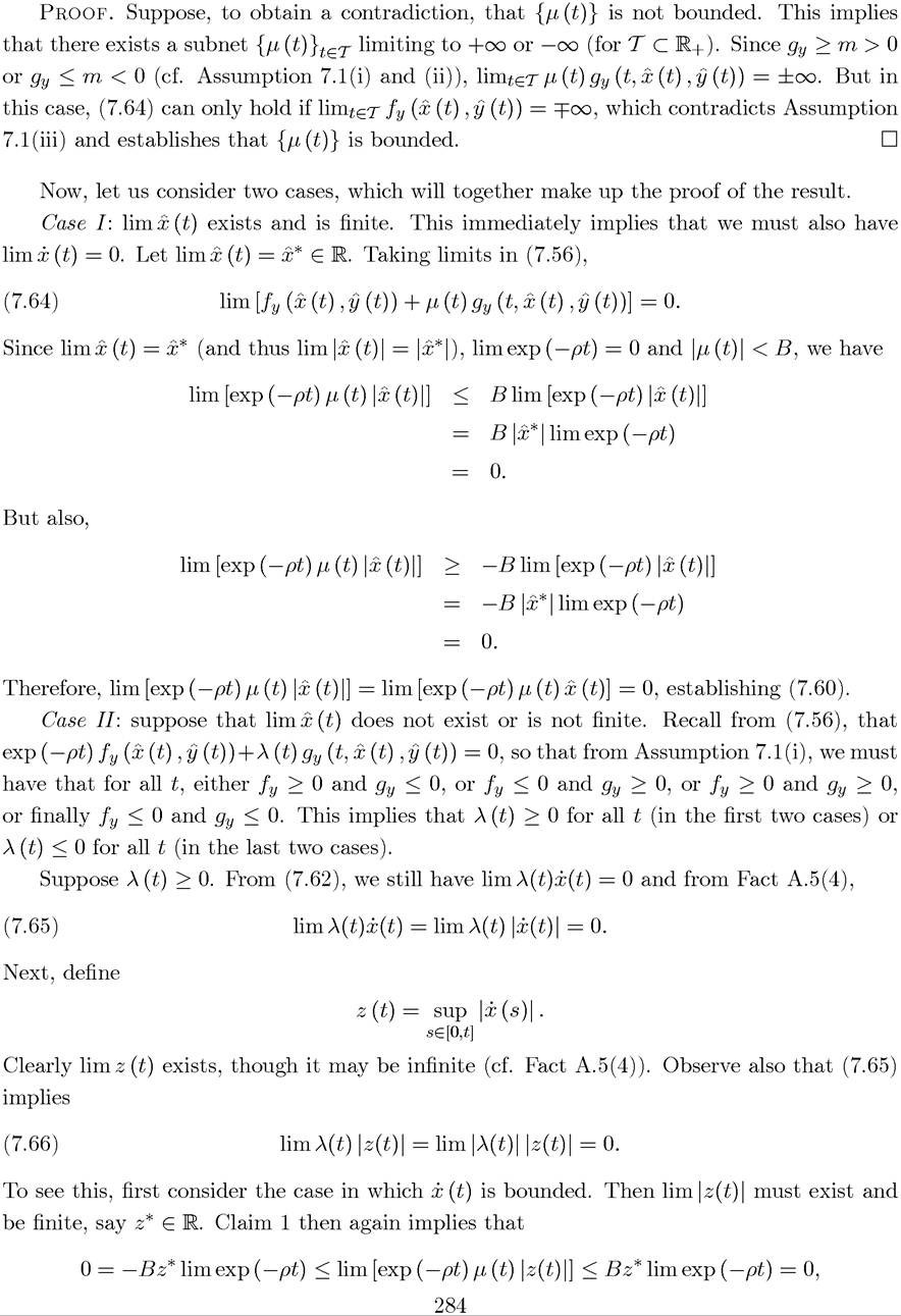
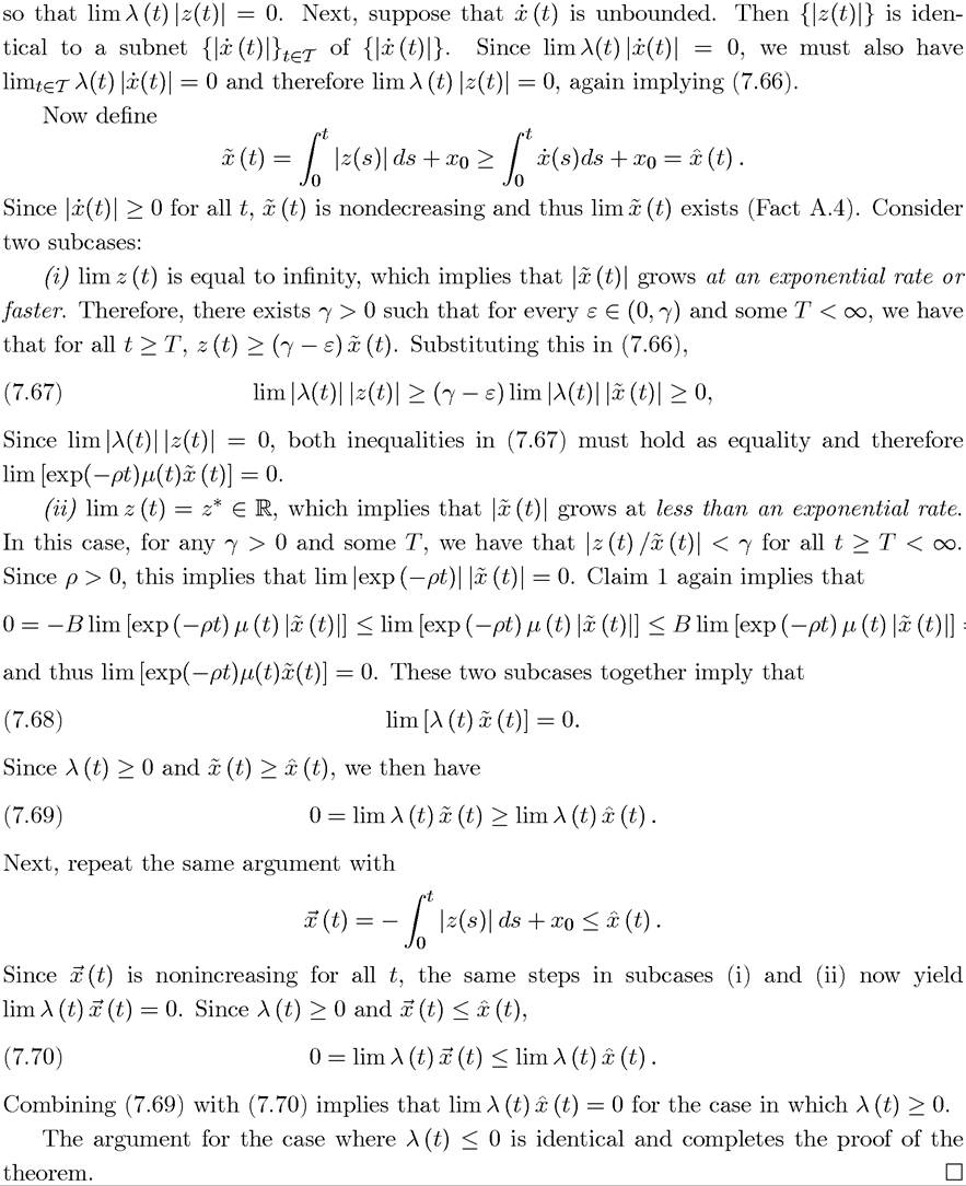
The proof of Theorem 7.13 also clarifies the importance of discounting. For example, neither the key equation, (7.64) nor the argument in subcase (ii) in the proof apply without discounting. Exercise 7.17 discusses how a similar result can be established without discounting under stronger assumptions. Exercise 7.20, on the other hand, shows why Assumption 7.1(iii) is necessary. This condition will be the harder one to verify in some economic models, 285
though in all models studied in the rest of the book we can make sure that it is satisfied and thus the current version of Theorem 7.13 can be applied directly in all of these cases.

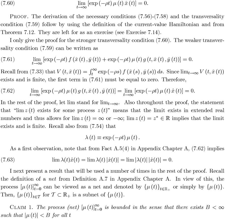
It is important to emphasize that Theorem 7.13 only provides necessary conditions for interior continuous solutions. In this light, (7.60) should be interpreted as a necessary transver- sality condition for such a solution. This implies that (7.60) is neither necessary (the solution may not be interior or continuous) nor sufficient. However, the next theorem shows that under the appropriate concavity conditions (7.60) is also a sufficient transversality condition.
More remarkably, it also shows that for concave problems, Assumption 7.1 is no longer necessary, thus, in concave problems, we can use (7.60) without having to check Assumption 7.1. Therefore, the next theorem will be the most important result of this chapter and will be used repeatedly in applications.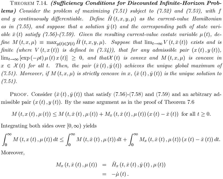
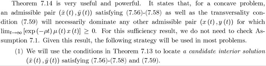
(2) We will then verify the concavity conditions of Theorem 7.14 and then simply check that for other admissible pairs. If these conditions
are satisfied, we will have characterized a global maximum.
An important feature of this theorem and the strategy outlined here is that they can be directly applied to unbounded problems (for example, to endogenous growth models). Therefore, as long as the conditions of Theorem 7.14 are satisfied, there is no need to make boundedness assumptions to characterize household behavior or optimal growth solutions.
7.6.