Existence of Solutions, Concavity and Differentiability*
The theorems presented so far characterize the properties of a solution to a continuoustime maximization problem. The natural question of when a solution exists has not been posed or answered so far.
This might appear curious, since both in finite-dimensional and in discrete-time infinite-horizon optimization problems studied in the previous chapter the analysis starts with existence theorems. There is a good reason for this omission, however. In continuous-time optimization problems, establishing existence of solutions is considerably more difficult than the characterization of solutions. I now present the general theorem on existence of solutions to continuous-time optimization problems and two additional results providing conditions under which the value function V (t,x), de fined in eq. (7.31) and Lemma 7.1, is concave and differentiable.The reader may have already wondered how valid the approach of using the necessary conditions provided so far, which did not verify the existence of a solution, would be in practice. This is an important concern, and ordinarily such an approach would open the door for potential mistakes. One line of defense, however, is provided by the sufficiency theorems, for example, Theorems 7.11 or 7.14 for infinite-horizon problems. If, given a continuous-time optimization problem, we find an admissible pair (X (t),y (t)) that satisfies the necessary conditions (e.g., those in Theorem 7.9) and we can then verify that the optimization problem satisfies the conditions in any one of Theorems 7.11 or 7.14, then we must have characterized an optimal solution and can dispense with an existence theorem. Therefore, the sufficiency results contained in these theorems enable us to bypass the step of checking for the existence of a solution. Nevertheless, this is only valid when the problem possesses sufficient concavity to satisfy the conditions of Theorems 7.11 or 7.14.
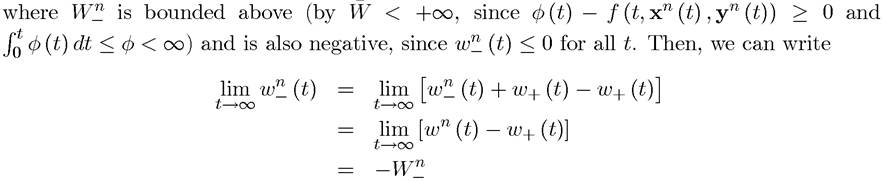
For problems that do not fall into this category, the justification for using the necessary conditions is much weaker. For this reason, and to provide a more complete treatment of continuous-time optimization problems, in this section I present an existence theorem for optimal control problems. Unfortunately, however, existence theorems for this class of problems are both somewhat complicated to state and difficult to prove. In particular, they require both measure-theoretic ideas and more advanced tools (some of them stated in the starred section, Section A.5, of Appendix Chapter A). I therefore provide a sketch of the proof of one of the most useful and powerful theorems, but I only give a sketch of some of the measure-theoretic details.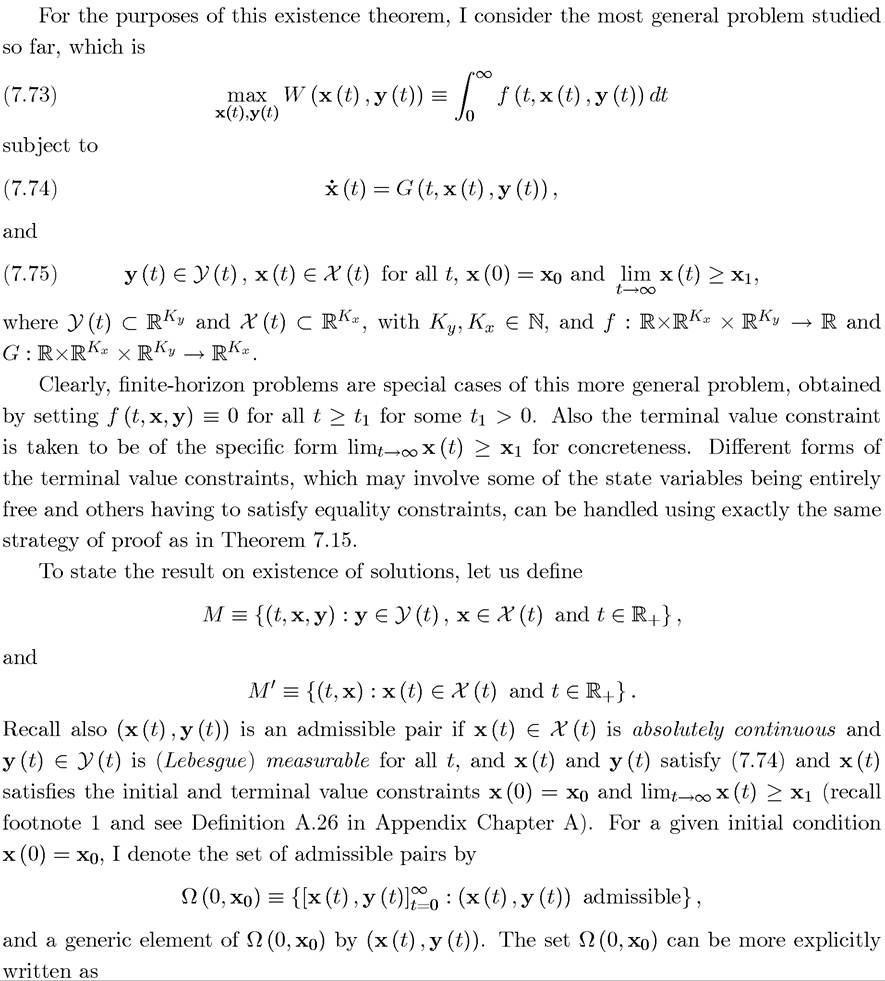
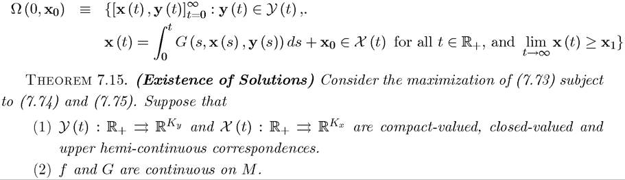
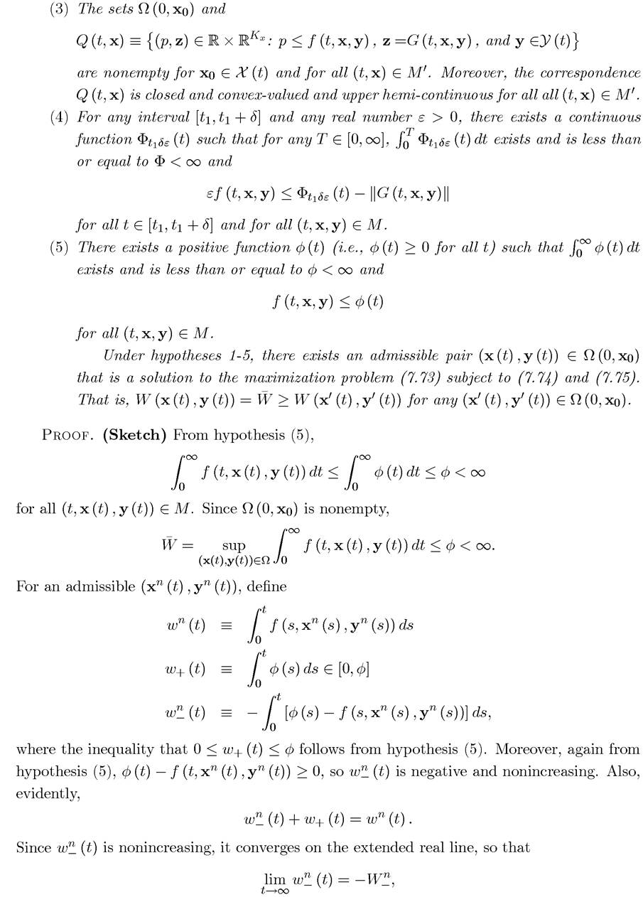
Theorem 7.15 establishes the existence of solutions to continuous-time maximization problems under relatively mild assumptions (at least from an economic point of view). Hypotheses (1) and (2) are the usual compactness and continuity assumption, necessary in finitedimensional and discrete-time optimization problems as well (recall, for example, Theorem A.9 in Appendix Chapter A). Hypotheses (4) and (5) are somewhat stronger versions of the boundedness assumptions that are also necessary in finite-dimensional and discrete-time optimization problems (these are sometimes referred to as “growth conditions” since they restrict the rate at which the objective function can grow).
Hypothesis (3) is rather unusual. Such a convexity assumption is not necessary in finite-dimensional and discrete-time optimization problems. However, in continuous-time problems this assumption cannot be dispensed with (see Exercise 7.24).While Theorem 7.15 establishes the existence of solutions, providing sufficient conditions for the solution (the control y (t)) to be continuous turns out to be much harder. Without knowing that the solution is continuous, the necessary conditions in Theorems 7.9 and/or 7.13 may appear incomplete. Although there is some truth to this, recall that both Theorems 7.9 and 7.13 provided necessary conditions only for all t except those at which y (t) is discontinuous. Therefore, these theorems remain valid as stated. Moreover, most economic problems possess enough structure to ensure that y (t) is continuous and x (t) is smooth. For example, in many economic problems Inada-type conditions ensure that optimal controls remain within the interior of the feasible set and concavity rules out discontinuous controls. However, instead of using these conditions to prove existence of continuous solutions, the indirect approach outlined above turns out to be more useful. In particular, in most economic problems the following approach works: (i) characterize a solution that satisfies the necessary conditions in Theorem 7.9 or in Theorem 7.13 (provided that such a solution exists); and (ii) verify the sufficiency conditions in one of Theorems 7.11 or 7.14. This approach, when it works, guarantees both the existence of a solution and continuity of the control (and smoothness of the state variable). Since all the problems in this book satisfy these conditions, this approach will be the one I will adopt in the remainder.
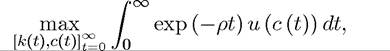
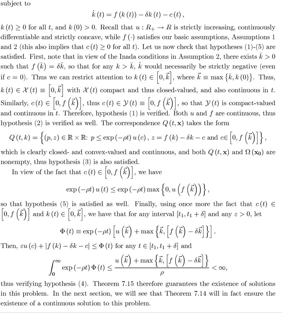
Let us next discuss how the conditions of Theorem 7.15 can be verified in the context of the optimal growth example, which will be discussed in greater detail in the next section.
Example 7.4. Consider the problem
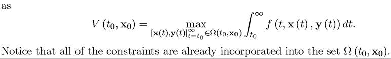
I next briefly present conditions under which the value function V (t, x) is concave and differentiable. Recall the definition of V (t, x) in (7.31), which was done for the case of a onedimensional state variable. Let us consider the more general problem of maximizing (7.73) subject to (7.74) and (7.75). Presuming that the solution exists, the value function is defined
7.7.