A First Look at Optimal Growth in Continuous Time
In this section, I briefly show how the main results developed so far, Theorems 7.13 and 7.14, can be applied to the problem of optimal growth. Recall that the optimal growth problem involves the maximization of the utility of the representative household.
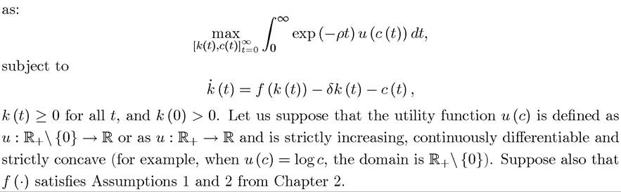
I do not provide a full treatment of this model here, since this is the topic of the next chapter. My objective is to illustrate how Theorems 7.13 and 7.14 can be applied in economic growth problems by using this canonical problem. I will show that checking the conditions for Theorem 7.13 requires some work, while verifying the conditions for Theorem 7.14 is much more straightforward.Consider the neoclassical economy without any population growth and without any technological progress. In this case, the optimal growth problem in continuous time can be written
Let us first set up the current-value Hamiltonian, which, in this case, does not directly depend on time and can be written as

with state variable k, control variable c and current-value costate variable μ.
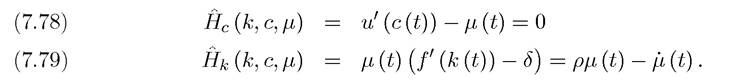
From Theorem 7.13, let us look for a path of capital stock and consumption per capita that satisfies the necessary conditions,
In addition, we would like to use the stronger transversality condition (7.60), which here takes the form

If we wish to show that this transversality condition is necessary (for an interior solution), we need to verify that Assumption 7.1 is satisfied. First, the objective function u (c) is increasing in c and independent of k, so it is weakly monotone. The constraint function, f (k) — δk — c, 
7.8.