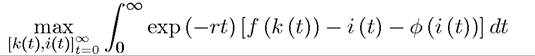
The q-Theory of Investment and Saddle-Path Stability

As another application of the methods developed in this chapter, I now consider the canonical model of investment under adjustment costs, also known as the q-theory of invest­ment.

The economic problem is that of a price-taking firm trying to maximize the present discounted value of its profits. The only twist relative to the problems studied so far is that this firm is subject to “adjustment” costs when it changes its capital stock. In particular, let the capital stock of the firm be k (t) ≥ 0 and suppose that the firm has access to a production function f (k) that satisfies Assumptions 1 and 2. For simplicity, let us normalize the price of the output of the firm to 1 in terms of the final good at all dates. The firm is subject to adjustment costs captured by the function φ (i), which is strictly increasing, continuously differentiable and strictly convex, and satisfies φ (0) = φ⁰ (0) = 0. This implies that in addition to the cost of purchasing investment goods (which given the normalization of price is equal to i for an amount of investment i), the firm incurs a cost of adjusting its production structure given by the convex function φ (i). In some models, the adjustment cost is taken to be a function of investment relative to capital—φ (i/k) instead of φ (i)—but this makes no difference for our main focus. I also assume that installed capital depreciates at an exponential rate δ and that the firm maximizes its net present discounted earnings with a discount rate equal to the interest rate r, which is assumed to be constant.

The firm’s problem can be written as

subject to

and k (t) ≥ 0, with k (0) > 0 given. Notice that φ (i) does not contribute to capital accu­mulation; it is simply a cost. Moreover, since φ is strictly convex, it implies that it is not 298

optimal for the firm to make “large” adjustments. Therefore it will act as a force towards a smoother time path of investment.

To characterize the optimal investment plan of the firm, let us use the same strategy as in the previous section. In particular, let us write the current-value Hamiltonian:

where I used q (t) instead of the familiar μ (t) for the costate variable, for reasons that will be apparent soon.

The necessary conditions for an interior solution to this problem, including the transver- sality condition, can be written as

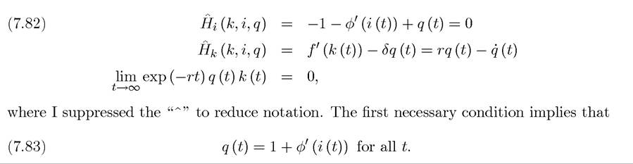
Let us next check sufficiency. Since q (t) > 0 for all t, H is strictly concave. Moreover, since k (t) ≥ 0 by feasibility, we also havefor any feasible

investment and capital stock process. Consequently, Theorem 7.14 applies and shows that a solution to (7.82) characterizes the unique profit-maximizing investment and capital stock process. Once again, it turns out that using Theorem 7.14 is both straightforward and powerful. In particular, the transversality condition corresponding to (7.60) is being used as a sufficient condition and there is no need to check Assumption 7.1.

Next, differentiating (7.83) with respect to time,

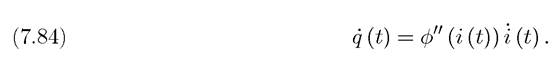
Substituting this into the second necessary condition, we obtain the following law of motion for investment:

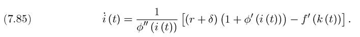
A number of interesting economic features emerge from this equation.

The behavior of investment and capital stock can now be analyzed using the differential equations (7.81) and (7.85). First, it can be verified easily that there exists a unique steady­state solution with ê > 0. This solution involves a level of capital stock k* for the firm and investment just enough to replenish the depreciated capital, i* = δk*. This steady-state level of capital satisfies the first-order condition (corresponding to the right-hand side of (7.85) being equal to zero):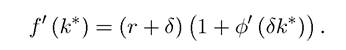

This first-order condition differs from the standard “modified golden rule” condition, which requires the marginal product of capital to be equal to the interest rate plus the depreciation rate, because an additional cost of having a higher capital stock is that there will have to be more investment to replenish depreciated capital. This is captured by the term φ⁰ (δk*). Since φ is strictly convex and f is strictly concave and satisfies the Inada conditions (from Assumption 2), there exists a unique value of k* that satisfies this condition.

The analysis of dynamics in this case requires somewhat different ideas than those used in the basic Solow growth model (cf., Theorems 2.4 and 2.5).

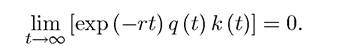
This implies that in the context of the current theory, with one state and one control variable, we should have a one-dimensional manifold (a curve) along which capital-investment pairs tend towards the steady state. This manifold is also referred to as the “stable arm”. The initial value of investment, i (0), will then be determined so that the economy starts along this curve. In fact, if any capital-investment pair (rather than only pairs along this curve) were to lead to the steady state, we would not know how to determine i (0); in other words, there would be an “indeterminacy” of equilibria. Mathematically, rather than requiring all eigenvalues of the linearized system to be negative, what we require now is saddle-path stability, which involves the number of (strictly) negative eigenvalues to be the same as the number of state variables.

This notion of saddle path stability is central in most growth models. Let us now make these notions more precise by considering the following generalizations of Theorems 2.4 and 2.5 (see Appendix Chapter B):

Theorem 7.18. (Saddle-Path Stability in Linear Systems) Consider the following linear differential equation system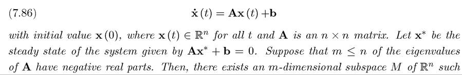

that starting from any x (0) ∈ M, the differential equation (7.86) has a unique solution with

Theorem 7.19. (Saddle-Path Stability in Nonlinear Systems) Consider the fol­lowing nonlinear autonomous differential equation

where G : Rⁿ → Rⁿ and suppose that G is continuously differentiable, with initial value x (0).

and suppose that m ≤ n of the eigenvalues of A have (strictly) negative real parts and the rest have (strictly) positive real parts. Then, there exists an open neighborhood of x*, B (x*) C Rⁿ and an m-dimensional manifold M C B (x*) such that starting from any x (0) ∈ M, the differential equation (7.87) has a unique solution with x (t) → x*.

Put differently, these two theorems state that when only a subset of the eigenvalues have negative real parts, a lower-dimensional subset of the original space leads to stable solutions. Fortunately, in this context this is exactly what we require, since i (0) should adjust in order to place us on exactly such a lower-dimensional subset of the original space.

Armed with these theorems, we can now investigate the transitional dynamics in the q-theory of investment. To see that the equilibrium will tend to this steady-state level of capital stock, let us to plot (7.81) and (7.85) in the k-i space. This is done in Figure 7.1. The curve corresponding tois upward sloping, since a greater level of capital

stock requires more investment to replenish the depreciated capital. When we are above this curve, there is more investment than necessary for replenishment, so that ê > 0. When we are below this curve, then ê < 0. On the other hand, the curve corresponding to i = 0, (7.85), can be nonmonotonic. Nevertheless, it is straightforward to verify that in the neighborhood of the steady-state it is downward sloping (see Exercise 7.28). When we are to the right of this curve, f⁰ (k) is lower, thus i > 0. When we are to its left, i < 0. The resulting phase diagram, together with the one-dimensional stable manifold, is shown in Figure 7.1 (see again Exercise 7.28 for a different proof).

We will next see that starting with an arbitrary level of capital stock, k (0) > 0, the unique optimal solution involves an initial level of investment i (0) > 0, followed by a smooth and monotonic approach to the steady-state investment level of δk*. In particular, it can be shown easily that when k (0) < ê *, i (0) > i * and it monotonically decreases towards i* (see Exercise 7.28). This is intuitive. Adjustment costs discourage large values of investment, thus the firm cannot adjust its capital stock to its steady-state level immediately. However, because of diminishing returns, the benefit of increasing the capital stock is greater when the level of capital stock is low. Therefore, at the beginning the firm is willing to incur greater adjustment costs in order to increase its capital stock and i (0) is high. As capital

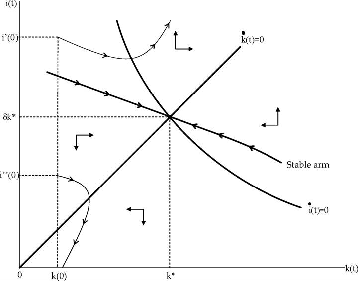
FIGURE 7.1. Dynamics of capital and investment in the q-theory.

accumulates and k (t) > ê (0), the benefit of boosting the capital stock declines and the firm also reduces investment towards the steady-state investment level.

There are two ways to see why the solution starting with (k (0),i (0)) and converging to (k*,i*) as shown in Figure 7.1 is the unique optimal solution. The first one, which is more rigorous and straightforward, is to use Theorem 7.14. As noted above, the conditions of this theorem hold in this problem. Thus we know that a path of capital and investment that satisfies the necessary conditions (that is, a path starting with (k (0),i (0)) and converging to (k*,i*)) is the unique optimal path. By implication, other paths, for example, those that start in i' (0) or i" (0) in Figure 7.1, cannot be optimal.

The second argument is common in the literature, though it is somewhat less complete than the argument just given. It involves showing that initial investment levels other than i (0) would violate either the transversality condition or the first-order necessary conditions. Consider, for example,as the initial level of investment. The phase diagram

in Figure 7.1 makes it clear that starting from such a level of investment, the necessary conditions imply that i (t) and k (t) would tend to infinity. It can be verified that in this

case q (t) k (t) would tend to infinity at a rate faster than r, thus violating the transversality condition,_ To see this more explicitly, note that along a

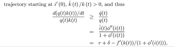
where the second line uses (7.83) and (7.84), while the third line substitutes from (7.85). As 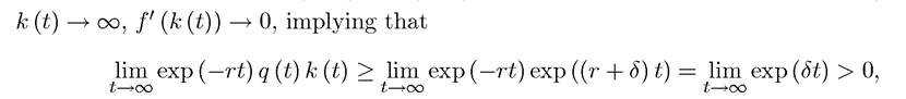violating the transversality condition. In contrast, if we start with i" (0) < i (0) as the initial level, i (t) would tend to 0 in finite time (as shown by the fact that the trajectories hit the horizontal axis) and k (t) would also tend towards zero (though not reaching it in finite time). After the time where i (t) = 0, we also have q (t) = 1 and thus q (t) = 0 (from (7.83)). Moreover, by the Inada conditions, as k (t) → 0, f (k (t)) → ∞. Consequently, after i (t) reaches 0, the necessary conditionis violated. This

establishes that the unique optimal path involves investment starting at i (0). The reason why this argument is not fully rigorous is that it is exploiting the necessary conditions for an interior continuous solution. However, when i (0) = 0, we are no longer in the interior of the feasibility set for the control variableand we cannot be sure that the necessary

conditions still apply. Despite the fact that this argument is not complete, it is often used in many different contexts and especially in the analysis of competitive growth problems. Therefore, I will outline how a similar argument can be developed for the neoclassical growth model in the next chapter, though the main tool of analysis will again be the sufficiency result in Theorem 7.14.

Let us next turn to the “q-theory” aspects. James Tobin argued that the value of an extra unit of capital to the firm divided by its replacement cost is a measure of the “value of investment to the firm”. In particular, when this ratio is high, the firm would like to invest more. In steady state, the firm will settle where this ratio is 1 or close to 1. In our formulation, the costate variable q (t) measures Tobin’s q. To see this, let us denote the current (maximized) value of the firm when it starts with a capital stock of k (t) by V (k (t)). The same arguments as above imply that

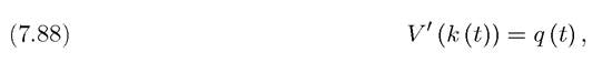
so that q (t) measures exactly by how much one dollar increase in capital will raise the value of the firm.

which is approximately equal to 1 when φ' (δk*) is small. Nevertheless, out of steady state, q (t) can be significantly greater than

this amount, signaling that there is need for greater investments. Therefore, in this model Tobin’s q, or alternatively the costate variable q (t), will signal when investment demand is high.

The q-theory of investment is one of the workhorse models of macroeconomics and finance, since proxies for Tobin’s q can be constructed using stock market prices and book values of firms. When stock market prices are greater than book values, this corresponds to periods in which the firm in question has a high Tobin’s q—meaning that the value of installed capital is greater than its replacement cost, which appears on the books. Nevertheless, whether this is a good approach in practice is intensely debated, in part because Tobin’s q does not contain all the relevant information when there are irreversibilities or fixed costs of investment, and also perhaps more importantly, what is relevant in theory (and in practice) is the “marginal q,” which corresponds to the marginal increase in value (as suggested by eq. (7.88)). However, in the data most measures compute “average q”. The discrepancy between these two concepts can be large.

7.9.