Transitional Dynamics
Next, we can determine the transitional dynamics of this model. Recall that transitional dynamics in the basic Solow model were given by a single differential equation with an initial condition.
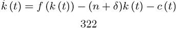
This is no longer the case, since the equilibrium is determined by two differential equations, repeated here for convenience: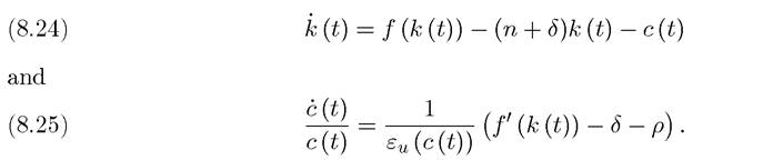
Moreover, we have an initial condition k (0) > 0, also a boundary condition at infinity, of the form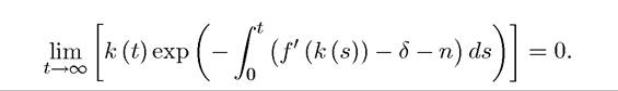
As we already discussed in the context of the q-theory of investment, this combination of an initial condition and a transversality condition is quite typical for economic optimal control problems where we are trying to pin down the behavior of both state and control variables. This means that we will again use the notion of saddle-path stability introduced in Theorems 7.18 and 7.19 instead of those in Theorems 2.4, 2.5 and 2.6. In particular, the consumption level (or equivalently the costate variable μ) is the control variable, and its initial value c (0) (or equivalently μ (0)) is free. It has to adjust so as to satisfy the transversality condition (the boundary condition at infinity). Since c (0) or μ (0) can jump to any value, we again need that there exists a one-dimensional curve (manifold) tending to the steady state. In fact, as in the q-theory of investment, if there were more than one paths tending to the steady state, the equilibrium would be indeterminate, since there would be multiple values of c(0) that could be consistent with equilibrium. Therefore, the correct notion of stability in models with state and control variables is one in which the dimension of the stable curve (manifold) is the same as that of the state variables, requiring the control variables jump on to this curve.
Fortunately, the economic forces are such that the correct notion of stability is guaranteed and indeed there will be a one-dimensional manifold of stable solutions tending to the unique steady state. There are two ways of seeing this. The first one simply involves studying the above system diagrammatically. This is done in Figure 8.1.
The vertical line is the locus of points where c = 0. The reason why the c = 0 locus is just a vertical line is that in view of the consumer Euler equation (8.25), only the unique level of k* given by (8.21) can keep per capita consumption constant. The inverse U-shaped curve is the locus of points where k = 0 in (8.24). The intersection of these two loci defined the steady state. The shape of the k = 0 locus can be understood by analogy to the diagram where we discussed the golden rule in Chapter 2. If the capital stock is too low, steady-state consumption is low, and if the capital stock is too high, then the steady-state consumption is again low. There exists a unique level, kgold that maximizes the state-state consumption per capita. The c = 0 locus intersects the k = 0 locus always to the left of kgold (see Exercise 8.8). Once these two loci are drawn, the rest of the diagram can be completed by looking at the direction of motion according to the differential equations. Given this direction of movements, it is clear that there exists a unique stable arm, the one-dimensional manifold tending to the steady state. All points away from this stable arm diverge, and eventually reach zero consumption or zero capital stock as shown in the figure. To see this, note that if initial consumption, c (0), started above this stable arm, say at c0 (0), the capital stock would reach 0 in finite time, while consumption would remain positive. But this would violate feasibility. Therefore, initial values of consumption above this stable arm cannot be part of the equilibrium (or the optimal growth solution).
If the initial level of consumption were below it, for example, at c00 (0), consumption would reach zero, thus capital would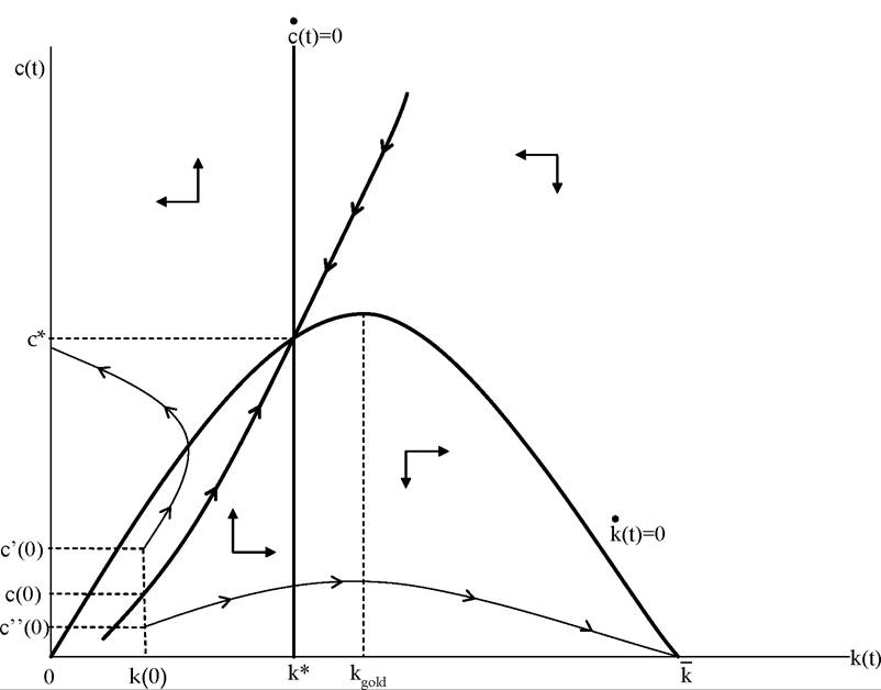
FIGURE 8.1. Transitional dynamics in the baseline neoclassical growth model.
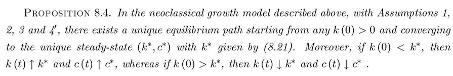
accumulate continuously until the maximum level of capital (reached with zero consumption) k > kgθid. Continuous capital accumulation towards with no consumption would violate the transversality condition. This establishes that the transitional dynamics in the neoclassical growth model will take the following simple form: c (0) will “jump” to the stable arm, and then (k, c) will monotonically travel along this arm towards the steady state. This establishes:
An alternative way of establishing the same result is by linearizing the set of differential equations, and looking at their eigenvalues. Recall the two differential equations determining the equilibrium path:
and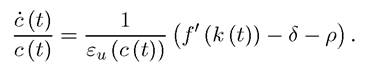
Linearizing these equations around the steady state (k*,c*), we have (suppressing time dependence)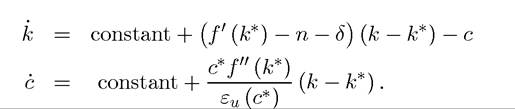
Moreover, from (8.21),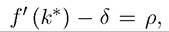 so the eigenvalues of this two-equation system are
given by the values of ξ that solve the following quadratic form:
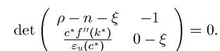
It is straightforward to verify that, since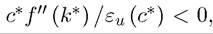 there are two real eigenval
ues, one negative and one positive. This implies that there exists a one-dimensional stable manifold converging to the steady state, exactly as the stable arm in the above figure (see Exercise 8.11). Therefore, the local analysis also leads to the same conclusion. However, the local analysis can only establish local stability, whereas the above analysis established global stability.
8.6.