Steady-State Equilibrium
Now let us characterize the steady-state equilibrium and optimal allocations. A steadystate equilibrium is defined as in Chapter 2 as an equilibrium path in which capital-labor ratio, consumption and output are constant.
Therefore,
From (8.20), this implies that as long as irrespective of the exact utility function,
we must have a capital-labor ratio k* such that

318
which is the equivalent of the steady-state relationship in the discrete-time optimal growth model.[20] This equation pins down the steady-state capital-labor ratio only as a function of the production function, the discount rate and the depreciation rate. This corresponds to the modified golden rule, rather than the golden rule we saw in the Solow model (see Exercise 8.8). The modified golden rule involves a level of the capital stock that does not maximize steady-state consumption, because earlier consumption is preferred to later consumption. This is because of discounting, which means that the ob jective is not to maximize steadystate consumption, but involves giving a higher weight to earlier consumption.
Given k*, the steady-state consumption level is straightforward to determine as:

which is similar to the consumption level in the basic Solow model. Moreover, given Assumption 40, a steady state where the capital-labor ratio and thus output are constant necessarily satisfies the transversality condition.
This analysis therefore establishes:
PROPOSITION 8.2.
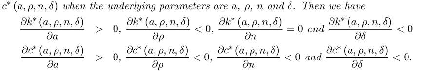
In the neoclassical growth model described above, with Assumptions 1, 2, 3 and 40, the steady-state equilibrium capital-labor ratio, k*, is uniquely determined by (8.21) and is independent of the utility function. The steady-state consumption per capita, c*, is given by (8.22).As with the basic Solow growth model, there are also a number of straightforward comparative static results that show how the steady-state values of capital-labor ratio and consumption per capita change with the underlying parameters. For this reason, let us again parameterize the production function as follows

where a > 0, so that a is again a shift parameter, with greater values corresponding to greater productivity of factors. Since f (k) satisfies the regularity conditions imposed above, so does

PROPOSITION 8.3. Consider the neoclassical growth model described above, with Assumptions and suppose that
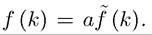 Denote the steady-state level of the
capital-labor ratio by k* (a, ρ, n, δ) and the steady-state level of consumption per capita by
Proof. See Exercise 8.5. ?
The new results here relative to the basic Solow model concern the comparative statics with respect the discount factor. In particular, instead of the saving rate, it is now the discount factor that affects the rate of capital accumulation. There is a close link between the discount rate in the neoclassical growth model and the saving rate in the Solow model. Loosely speaking, a lower discount rate implies greater patience and thus greater savings.
In the model without technological progress, the steady-state saving rate can be computed as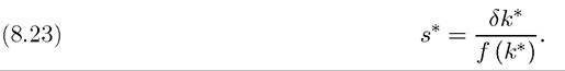
Exercise 8.7 looks at the relationship between the discount rate, the saving rate and the steady-state per capita consumption level.
Another interesting result is that the rate of population growth has no impact on the steady state capital-labor ratio, which contrasts with the basic Solow model. We will see in Exercise 8.4 that this result depends on the way in which intertemporal discounting takes place. Another important result, which is more general, is that k* and thus c* do not depend on the instantaneous utility function u (∙). The form of the utility function only affects the transitional dynamics (which we will study next), but has no impact on steady states. This is because the steady state is determined by the modified golden rule. This result will not be true when there is technological change, however.
8.5.