Transitional Dynamics
As already discussed in the context of the q-theory of investment, this combination of boundary conditions consisting of an initial condition and a transversality condition is quite typical for economic optimal control problems involving the behavior of both state and control variables.
The appropriate notion of stability is again that of saddle-path stability introduced in Theorems 7.18 and 7.19 (instead of the global stability results in Theorems 2.4 and 2.5). In particular, the consumption level (or equivalently the costate variable μ) is the control variable, and its initial value c (0) (or equivalently μ (0)) is free. It has to adjust so as to satisfy the transversality condition (the boundary condition at infinity). Since c (0) or μ (0) can jump to any value, we again need that there exists a unique one-dimensional manifold (curve) tending to the steady state. As in the q-theory of investment, if there were more than one paths tending to the steady state, the equilibrium would be indeterminate, since there would be multiple values of c(0) that could be consistent with equilibrium.Fortunately, the economic forces are such that once we use the correct notion (saddlepath stability), stability is guaranteed and also there exists a unique competitive equilibrium path. In particular, in the neoclassical growth model there exists a one-dimensional manifold (curve) of stable solutions, often referred to as the stable arm, tending to the unique steady state. This can be seen in Figure 8.1. The vertical line is the locus of points where The reason why the c = 0 locus is just a vertical line is that in view of the consumer Euler equation (8.38), only the unique level of k* given by (8.34) can keep per capita consumption constant.
 in (8.37). The intersection of these two loci de fines the steady state (k*,c*). The shape of the
 locus can be understood by analogy to the diagram where we discussed the golden rule in Chapter 2. If the capital stock is too low, steady-state consumption is low, and if the capital stock is too high, then the steady-state consumption is again low. There exists a unique level,
 kgθid that maximizes the steady-state consumption per capita. The c = 0 locus intersects the k = 0 locus always to the left of kgθid (see Exercise 8.17). Once these two loci are drawn, the rest of the diagram can be completed by looking at the direction of motion according to the differential equations, (8.37) and (8.38). Given this direction of movements, it is clear that there exists a unique stable arm tending to the steady state. This implies that starting with an initial capital-labor ratio k (0) > 0, there exists a unique c (0) on the stable arm. If the representative household starts with a per capita consumption level of c (0) at date t = 0 and then follows the consumption path given by the Euler equation (8.38), consumption per capita and the capital-labor ratio will converge to the unique steady state (k*,c*).
Is the path starting with (k (0),c (0)) and converging to (k*,c*) the unique equilibrium? The answer is yes and there are three ways of seeing this. The first one again involves a direct application of Theorem 7.14. In particular, we have already verified that the concavity
addition, no other path will provide the representative household with the same utility (see Exercise 8.11). Thus the path starting with (k (0),c (0)) is the unique competitive equilib
rium.
The same argument applies to the optimal growth problem, which is also described by the same equations. The path starting with (k (0),c (0)) is therefore the unique optimalgrowth path as well.
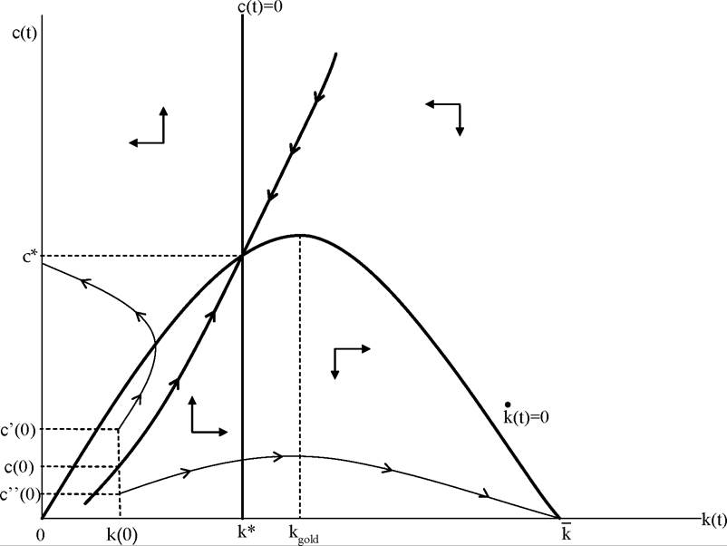
Figure 8.1. Transitional dynamics in the baseline neoclassical growth model.
The second strategy is the most popular in the literature and involves ruling out all paths other than the stable arm in Figure 8.1. In particular, Figure 8.1 makes it clear that all points away from the stable arm diverge, and eventually reach zero consumption or zero capital stock. For instance, if the initial level of consumption were below the stable arm, for example, at c00 (0), then consumption would reach zero in finite time, thus capital would accumulate continuously until the maximum level of capital (reached with zero consumption),  It can be verified that
 (see Exercise 8.12), which implies that

violating the transversality condition, (8.28) or (8.39). This implies that paths starting below the stable arm cannot be part of an equilibrium. Next, suppose that initial consumption starts above this stable arm, say at In this case, the capital stock would reach 0 in finite time, while household consumption implied by (8.38) would remain positive (see Exercise 8.12).3 But this violates feasibility and establishes that initial values of consumption above this
3
3There is the same technical problem here as the one pointed out in the context of the q-theory of investment in Section 7.8 in the previous chapter; when c reaches 0, the necessary conditions no longer apply.
stable arm cannot be part of the equilibrium (or the optimal growth solution).
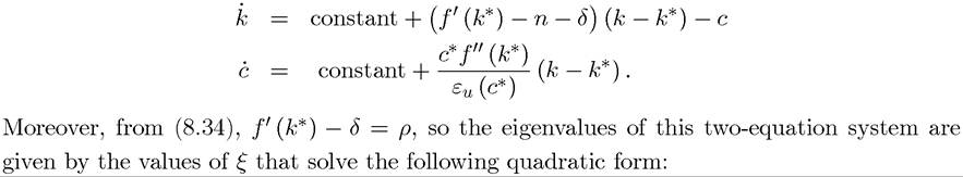
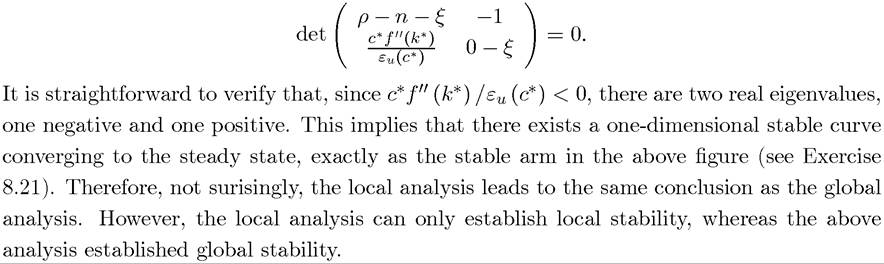
This line of argument then also leads to the conclusion that the transitional dynamics in the neoclassical growth model will involve the initial consumption per capita jumping to c (0) on the stable arm, and then (k, c) monotonically travel along this arm towards the steady state.Finally, the third way of establishing the same result is by linearizing the two differential equations characterizing the equilibrium path, (8.37) and (8.38). Linearizing these equations around the steady state (k*,c*) and suppressing time dependence, we obtain
8.6.