Neoclassical Growth in Discrete Time
It is useful to briefly discuss the baseline neoclassical growth model in discrete time to show the similarity of both the mechanics and the insights to the continuous-time analysis.
Discrete time equilibrium growth models will be discussed in greater detail in Chapter 17, when we introduce uncertainty.For now let us suppose that there is no population growth, so that c (t) denotes per capita consumption, the representative household inelastically supplies one unit of labor, and as usual, β ∈ (0,1) is the discount factor. The representative household then maximizes 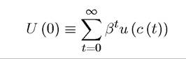 subject to the budget constraint

where a (t) is the asset holdings of the individual at time t, w (t) is the equilibrium wage rate, which is also equal to the labor income of the representative household, who supplies one unit of labor to the market, and r (t) is the rate of return on assets holdings at time t. As in the continuous-time model, this flow budget constraint needs to be augmented with a 333 no-Ponzi condition. With a similar reasoning to that which led to (8.14) in Section 8.1, this condition takes the form
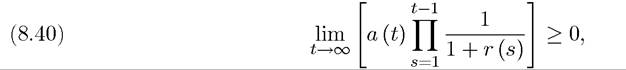
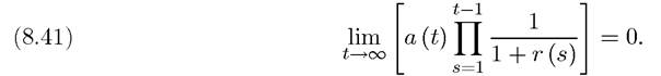
and ensures that the present discounted value of the representative household’s asymptotic debt is nonnegative (see Exercise 8.23). The representative household’s transversality condition then implies that a (t) cannot limit to a negative value, therefore the stronger form of the no-Ponzi condition, which must hold an equilibrium, is
The production side of the economy is identical to that in the continuous-time model.
Specifically, the rental rate of capital R (t) and the wage rate w (t) are given by (8.5) and(8.6). Moreover, given depreciation at the geometric rate δ > 0 in discrete time, the rate of return on assets, r (t), is again given by (8.26). Next, straightforward application of the results in Chapter 6 implies that the representative household will choose a consumption path that satisfies the Euler equation

The reader will recall from the analysis of optimal growth in discrete time in Section 6.8 in Chapter 6 that this is identical to the Euler equation for the optimal growth problem (since from (8.26) r (t) = f' (k (t)) — δ). To establish the equivalence of the competitive equilibrium and the optimal growth paths, we only need to show that the no-Ponzi condition (8.41) implies the transversality condition in the optimal growth problem (6.48) and vice versa. To see this, let us again use (8.26) to rewrite (6.48) as
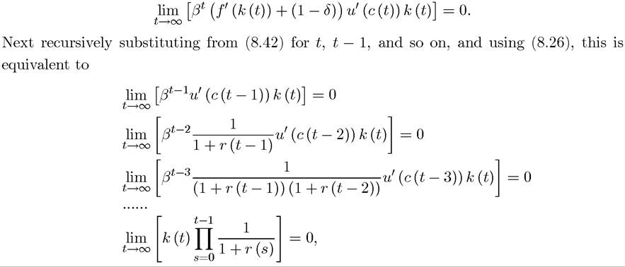
where the last line cancels out u' (c (0)), which is strictly positive by assumption. Since from market clearing a (t) = k (t), this condition is the same as (8.41) and thus establishes that the competitive equilibrium and optimal growth paths coincide. Naturally, this result is not 334
surprising, since the neoclassical growth model satisfies the conditions of the First and Second Welfare Theorems, Theorems 5.6 and 5.7. Nevertheless, the explicit derivation here shows how this equivalence manifests itself in the context of this workhorse model of growth theory and macroeconomics.
Given the equivalence between the equilibrium and optimal growth paths, Proposition 6.3 from Section 6.8 in Chapter 6 also characterizes the dynamics of the equilibrium allocation. In particular, this proposition implies that starting with any initial level of capital stock k (0) > 0, the competitive equilibrium path of the neoclassical growth model will monotonically converge to the unique steady-state allocation. This result therefore highlights the parallel between the general insights from the discrete-time and continuous-time models.
8.7.