Technological Change and the Canonical Neoclassical Model

The above analysis was for the neoclassical growth model without any technological change. As with the basic Solow model, the neoclassical growth model does not account for the long-run growth experience of the world economy without some type of exogenous technological change.

The production function is extended to:

(8.43) Y (t) = F [K (t),A (t) L (t)],

where

A (t) = exp (gt) A (0).

Notice that the production function (8.43) imposes purely labor-augmenting—Harrod- neutral—technological change. This is because Theorem 2.6 in Chapter 2 still applies and implies that balanced growth is only possible with technological change that is asymptotically labor-augmenting. As in that chapter, I simplify the analysis by assuming that technological change is labor-augmenting throughout.

Assumptions 1, 2 and 3 on the production and utility functions are still in effect. As­sumption 4⁰ will be strengthened further in order to ensure finite discounted utility in the presence of sustained economic growth.

The constant returns to scale feature again enables us to work with normalized variables.

Now let us define

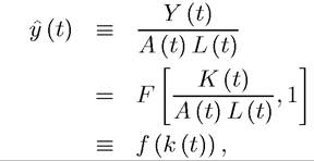
where

is the effective capital-labor ratio, written incorporating labor-augmenting technology in the denominator. Naturally, this is similar to the way that the effective capital-labor ratio was defined in the basic Solow growth model.

In addition to the assumptions on technology, we also need to impose a further assumption on preferences in order to ensure balanced growth.

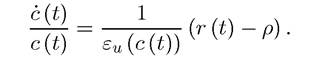
that is, if the elasticity of marginal utility of consumption is asymptotically constant. Therefore, balanced growth is only consistent with utility functions that have asymptotically constant elasticity of marginal utility of consumption. Since this result is important, I state it as a proposition:

PROPOSITION 8.5. Balanced growth in the neoclassical model requires that asymptotically (as t → ∞) all technological change is purely labor-augmenting and the elasticity of intertem­poral substitution, ε_u (c (t)), tends to a constant ε_u.

The next example shows the family of utility functions with constant intertemporal elas­ticity of substitution, which are also those with a constant coefficient of relative risk aversion.

Example 8.1. (CRRA Utility) Recall that the Arrow-Pratt coefficient of relative risk aversion for a twice differentiable concave utility function U (c) is

The constant relative risk aversion (CRRA) utility function satisfies the property that R is constant. Now integrating both sides of the previous equation, setting R to a constant, implies that the family of CRRA utility functions is given by

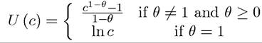
with the coefficient of relative risk aversion is given by θ (see Exercise B.9 in Appendix Chapter B for a formal derivation).

With time-separable utility functions, the inverse of the elasticity of intertemporal sub­stitution (defined in eq. (8.29)) and the coefficient of relative risk aversion are identical.

Therefore, the family of CRRA utility functions are also those with constant elasticity of intertemporal substitution.

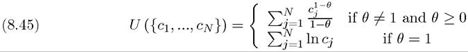
Now to link this utility function to the Gorman preferences discussed in Chapter 5, let us consider a slightly different problem in which an individual has preferences defined over the consumption of N commodities {c1,...,cn} given by

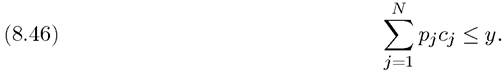
Suppose also that this individual faces a price vector p ≠(pι,...,Pn) and has income y, so that his budget constraint can be expressed as

Maximizing utility subject to this budget constraint leads to the following indirect utility

function

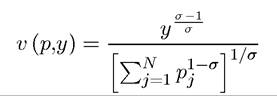
(see Exercise 5.6). Although this indirect utility function does not satisfy the Gorman form in Theorem 5.2, a monotonic transformation thereof does (simply raise it to the power σ/ (σ - 1)).

This establishes that CRRA utility functions are within the Gorman class, and if all indi­viduals have CRRA utility functions, then we can aggregate their preferences and represent them as if they belonged to a single individual.

Now consider a dynamic version of these preferences (defined over infinite horizon):

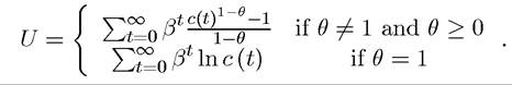
The important feature of these preferences in growth theory is not that the coefficient of rela­tive risk aversion is constant, but that the intertemporal elasticity of substitution is constant (since most of growth models do not feature uncertainty, but involve intertemporal allocation of consumption).

Given the restriction that balanced growth is only possible with preferences featuring a constant elasticity of intertemporal substitution, let us start with the CRRA instantaneous 337

utility function

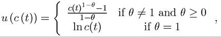
where the elasticity of marginal utility of consumption, ε_u, is given by the constant θ. When θ = 0, these represent linear preferences, whereas when θ = 1, they correspond to log prefer­ences. As θ → ∞, these preferences become infinitely risk-averse, and infinitely unwilling to substitute consumption over time.

More specifically, the economy now admits a representative household with CRRA pref­

erences

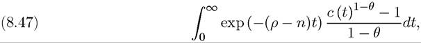
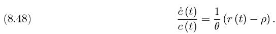
where c (t) ? C (t) /L (t) is per capita consumption. I refer to this model, with labor­augmenting technological change and CRRA preference as given by (8.47) as the canonical model, since it is the model used in almost all applications of the neoclassical growth model. In this model, the representative household’s problem is given by the maximization of (8.47) subject (8.8) and (8.14). Once again using the necessary conditions from Theorem 7.13, the Euler equation of the representative household is obtained as

Let us first characterize the steady-state equilibrium in this model with technological progress.

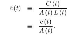
This normalized consumption level will remain constant along the BGP. In particular,

where recall that k (t) ? K (t) /A (t) L (t).

The transversality condition, in turn, can be expressed as

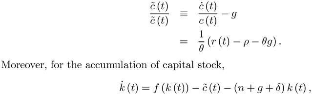
In addition, the equilibrium interest rate, r (t), is still given by (8.26). Moreover, since in steady state (BGP) c (t) must remain constant, r (t) = ρ + θg,which implies that

(8.50)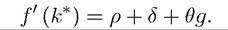

This equation pins down the steady-state value of the normalized capital ratio k* uniquely, in a way similar to the model without technological progress. The level of normalized consumption is then given by

while per capita consumption grows at the rate g.

The only additional complication in this case is that because there is now sustained growth, the transversality condition becomes more demanding. In particular, substituting

(8.50) into (8.49),

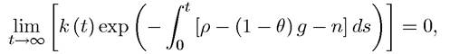
which can only hold if the integral within the exponent goes to zero, that is, only if ρ - (1 - θ) g - n > 0. This implies that to ensure a well-defined solution to the house­hold maximization problem and a well-defined competitive equilibrium, we need to modify Assumption 4⁰ to:

Assumption 4. (Discounting with Technological Progress)

Note that this assumption strengthens Assumption 4⁰ when θ < 1.

At this point, we can also use a similar reasoning to that in Section 8.2 and establish that, given Assumption 4, the sufficiency conditions in Theorem 7.14 are satisfied, so that the solution to the household maximization problem derived above indeed corresponds to a global maximum (see Exercise 8.18). In this light, the following is an immediate generalization of Proposition 8.2:

PROPOSITION 8.6. Consider the neoclassical growth model with labor-augmenting techno­logical progress at the rate g and preferences given by (8.f7). Suppose that Assumptions 1, 2, 3 and 4 hold. Then, there exists a unique BGP with a normalized capital to effective labor ratio of k*, given by (8.50), and output per capita and consumption per capita grow at the rate g.

The steady-state (BGP) capital-labor ratio is no longer independent of the utility function of the representative household, since now the steady-state capital-labor ratio, k* given by 339

(8.50), depends on the elasticity of marginal utility (or the inverse of the intertemporal elastic­ity of substitution), θ. This is because there is now positive growth in output per capita, and thus in consumption per capita. Since individuals face an upward-sloping consumption pro­file, their willingness to substitute consumption today for consumption tomorrow determines how much they will accumulate and thus the equilibrium effective capital-labor ratio.

Perhaps the most important implication of Proposition 8.6 is that, while the steady-state effective capital-labor ratio, k*, is determined endogenously, the steady-state growth rate of the economy is given exogenously and is equal to the rate of labor-augmenting technological progress, g. Therefore, the neoclassical growth model, like the basic Solow growth model, endogenizes the capital-labor ratio, but not the growth rate of the economy. The advantage of the neoclassical growth model is that the capital-labor ratio and the equilibrium level of (normalized) output and consumption are determined by the preferences of the individuals rather than an exogenously fixed saving rate. This also enables us to compare equilibrium and optimal growth (and in this case conclude that the competitive equilibrium is Pareto optimal and any Pareto optimum can be decentralized). But the determination of the rate of growth of the economy is still outside the scope of analysis.

A similar analysis to before also leads to a generalization of Proposition 8.4.

PROPOSITION 8.7. Consider the neoclassical growth model with labor-augmenting tech­nological progress at the rate g and preferences given by (8.47). Suppose that Assumptions

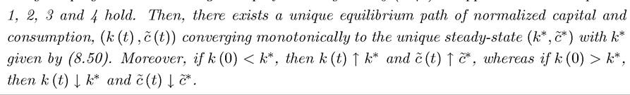
Proof. See Exercise 8.19. ?

It is also useful to briefly look at an example with Cobb-Douglas technology.

Example 8.2. Consider the model with CRRA utility and labor-augmenting technologi­cal progress at the rate g. Assume that the production function is given by F (K, AL) = and thusIn this case, suppressing time dependence to simplify notation, the

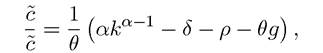
Euler equation written in terms of normalized consumption becomes

and the accumulation equation can be written as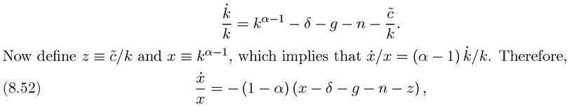

and also

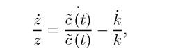
which implies that

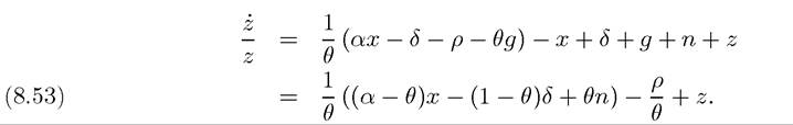
The two differential equations (8.52) and (8.53) together with the initial condition x (0) and the transversality condition completely determine the dynamics of the system. In Exercise 8.22, you are asked to complete this example for the special case in which θ → 1 (log preferences).

8.8.