CHAPTER C Brief Review of Dynamic Games

This chapter provides a very brief overview of some basic definitions, results and notation for infinite-horizon dynamic games. The reader is already assumed to be familiar with basic game theory, and the notions of Nash Equilibrium and Subgame Perfect Nash Equilibrium in finite games.

C. 1. Basic Definitions

I will consider the following class of dynamic infinite-horizon games. As the name sug­gests, these games are not finite and they are also somewhat more general than repeated games, since the stage game played at each date is a function of actions taken in the past.

More formally, there is a set of players denoted by N. This set will be either finite, or when it is infinite (especially uncountable), there will be more structure to make the game tractable and thus variants of the theorems here applicable. In particular, in many of the applications, especially in those considered in Chapters 22 and 23, there will be a continuum of players, but these will be in distinct finite groups and the game can be viewed as one between those distinct groups. With this motivation, in this Appendix I focus on the case in which N is finite, consisting of N players. Each player i ∈ N has a strategy set Ai (k) C Rⁿⁱ at every date, where k ∈ K C Rⁿ is the state vector, with value at time t denoted by k (t).

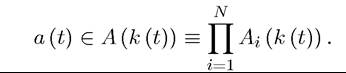
I use the standard notationto denote the vector

of actions without i’s action, thus we can also writeNotice that,

consistent with the types of models analyzed in the text, the action set of each player Ai (k) is only a function of the state variable k and not of calendar time.

Each player has an instantaneous utility function ù (a (t),k (t)) where

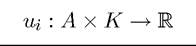
is assumed to be continuous and bounded. This notation emphasizes that each player’s payoff depends on the entire action profile in that period (and not on past actions) and also on a common vector of state variables, denoted by k (t). Past actions will only have an effect on current payoffs through this vector of state variables.

As usual, each player’s objective at time t is to maximize their discounted payoff

S 0

where β ∈ (0,1) is the discount factor and E_t is the expectations operator conditional on information available at time t. The games I focus on here have potential uncertainty about the evolution of the state variable in the future and also strategic uncertainty resulting because of mixed strategies. However, they will not feature asymmetric information, since I did not use incomplete information or asymmetric information dynamic games in this book. Consequently, the expectations operator E_t is not indexed by i.

The law of motion of the state vector k (t) is given by the following Markovian transition function

which denotes the probability density that next period’s state vector is equal to k (t + 1) when the time t action profile of all the agents is a (t) ∈ A (k (t)) and the state vector is k (t) ∈ K.

Next, we need to specify the information structure of the players. We focus on games with perfect observability or perfect monitoring, so that individuals observe realizations of all past actions (in case of mixed strategies, they observe realizations of actions not the strategies). Then, the public history at time t, observed by all agents up to time t, is therefore

the history of the game up to and including time t. With mixed strategies, the history would naturally only include the realizations of mixed strategies not the actual strategy. Let the 1180

set of all potential histories at time t be denoted by H^t. It should be clear that any element h^t ∈ H^t for any t corresponds to a subgame of this game.^[LVI]

Let a (pure) strategy for player i at time t be

i.e., a mapping that determines what to play given the entire past history h^t-1 and the current value of the state variable k (t) ∈ K. This is the natural specification of a strategy for time t given that h^t-1 and k (t) entirely determine which subgame we are in.

A mixed strategy for player i at time t is

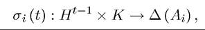
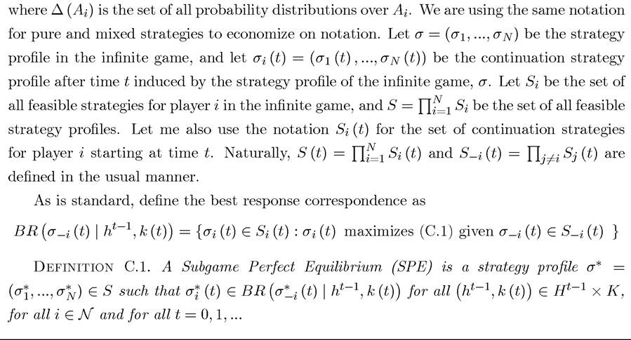
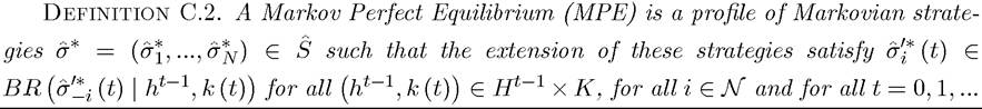
Therefore, a SPE requires strategies to be best responses to each other given all possible histories, which is a minimal requirement.

Perhaps the most popular alternative concept often used in dynamic games is that of Markov Perfect Equilibrium (MPE). The MPE differs from the SPE in only conditioning on the payoff-relevant “state”. The motivation comes from dynamic programming where, as we have seen, an optimal plan is a mapping from the state vector to the control vector. MPE can be thought of as an extension of this reasoning to game-theoretic situations. The advantage of the MPE relative to the SPE is that most infinite games will have many fewer MPEs tha SPEs in general. The disadvantage, naturally, is that some economically interesting SPEs will be ignored when we focus on MPEs.

We could define payoff relevant history at time t in general as the smallest partition of P^t of H^t such that any two distinct elements of P^t necessarily lead to different payoffs or strategy sets for at least one of the players holding the action profile of all other players constant.

In this case, it is clear that given the Markovian transition function above, the payoff relevant state is simply k (t) ∈ K. Then we define a pure Markovian strategy as and a mixed Markovian strategy as

Define the set of Markovian strategies for player i byand naturally,

Notice that I have dropped the t subscript here.

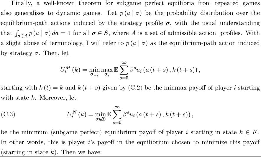
Let us next define:

C. 2. Some Basic Results

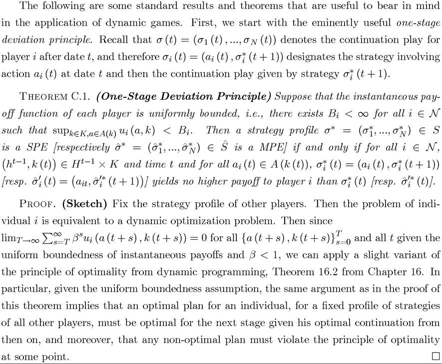
This theorem basically implies that in dynamic games, we can check whether a strategy is a best response to other players’ strategy profile by looking at one-stage deviations, keeping the rest of the strategy profile of the deviating player as given. The uniform boundedness assumption can be weakened to require “continuity at infinity”, which essentially means that discounted payoffs converge to zero along any history (and this assumption can also be relaxed further).

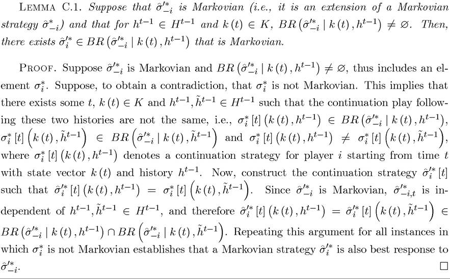
This lemma states that when all other players are playing Markovian strategies, there exists a best response that is Markovian for each player. This does not mean that there are no other best responses, but since there is a Markovian best response, this gives us hope in constructing Markov Perfect Equilibria. Consequently, we have the following theorem:

Existence of SPEs when K and Ai (k) are uncountable sets is much easier to guarantee.

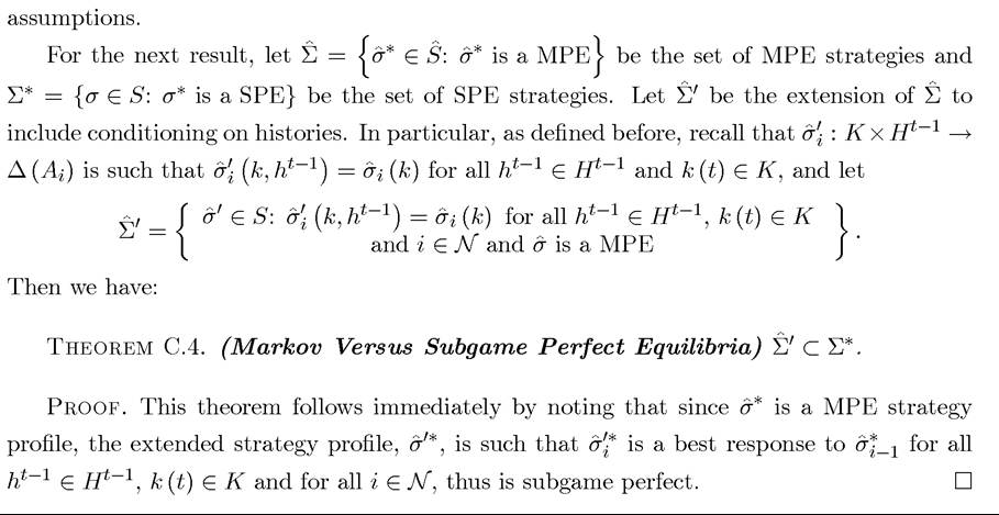
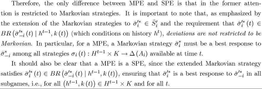
This theorem implies that every MPE strategy profile corresponds to a SPE strategy profile and any equilibrium-path play supported by a MPE can be supported by a SPE.

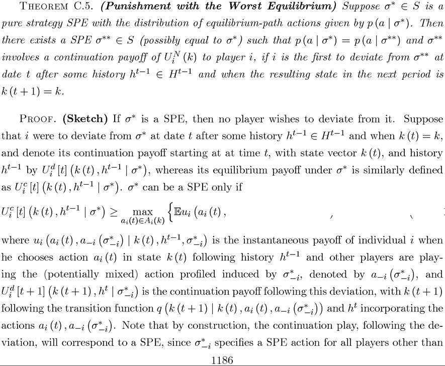
a-_i (σ*-i) | k (t),h^t~¹} + βEUf [t + 1] (k (t + 1),h^t | ⅛)1,

i in all subgames, and in response, the best that player i can do is to play an equilibrium strategy.

By definition of a SPE and the minimum equilibrium payoff of player i defined in (C.3), we have

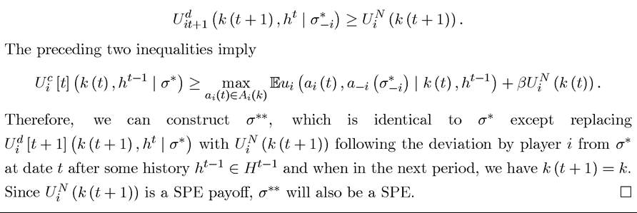
This theorem therefore states that when looking for the set of SPEs, we can limit attention to those involving the most severe equilibrium punishments.

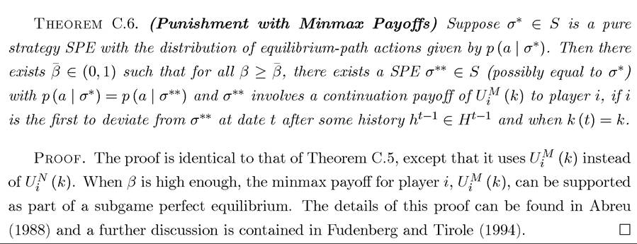
A stronger version of this theorem is the following:

C. 3. Application: Repeated Games With Perfect Observability

For repeated games with perfect observability, both SPE and MPE are easy to characterize and their properties are well-known. In particular, suppose that we have the same stage game played an infinite number of times, so that payoffs are given by

which is only different from (8.3) because there is no conditioning on the state variable k (t). Let us refer to the game {ui (a),a ∈ A } as the stage game. Define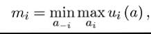

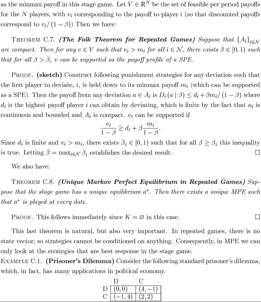
The stage game has a unique equilibrium, which is (D,D). Now imagine this game being repeated an infinite number of times with both agents having discount factor β. The unique MPE is playing (D,D) at every date.

In contrast, when β > 1/2, then (C,C) at every date can be supported as a SPE. To see this, recall that we only need to consider the minmax punishment, which in this case is (0, 0). Playing (C,C) leads to a payoff of 2/ (1 — β), whereas the best deviation leads to the payoff of 4 now and a continuation payoff of 0. Therefore, β > 1/2 is sufficient to make sure 1188

that the following grim strategy profile implements (C,C) at every date: for both players, the strategy is to play C if h^t includes only (C,C) and play D otherwise.

Why this strategy combination is not a MPE is also straightforward to see. The grim strategy ensures cooperation by conditioning on past history, i.e., it conditions on whether somebody has defected at any point in the past. This history is not payoff relevant for the future of the game given the action profile of the other player—fixing the action profile of the other player, whether somebody has cheated in the past or not has no effect on future payoffs.

C. 4. Exercises

EXERCISE C.1. A simple application of the ideas in this appendix are common pool games. Consider a society consisting of N + 1 < ∞ players each with payoff function

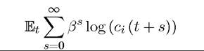
at time t where β ∈ (0,1) and Ci (t) denotes consumption of individual i ∈ N at time t. The society has a common resource, denoted by K (t), which can be thought of as the capital stock at time t. This capital stock follows the non-stochastic law of motion: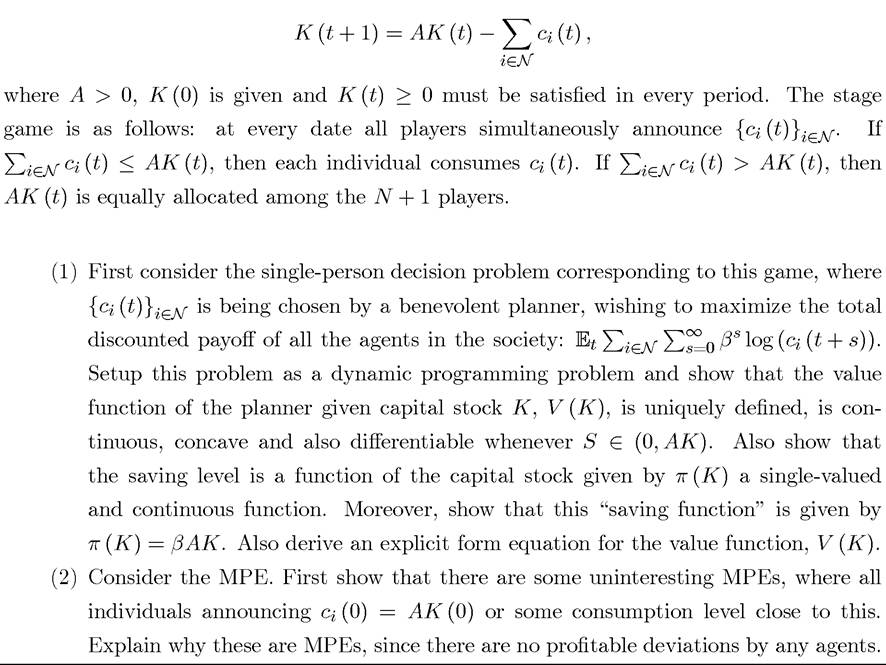

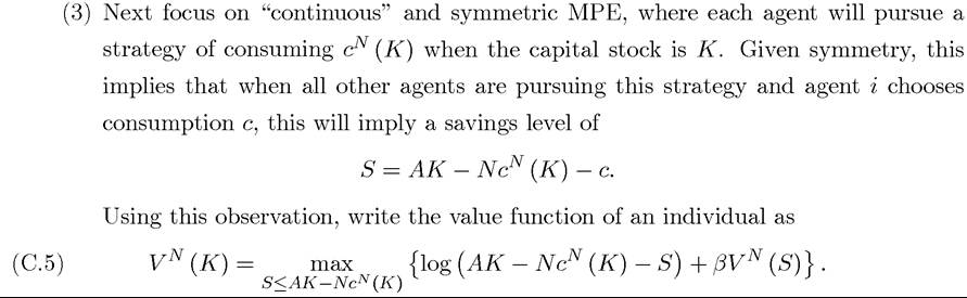
Explain this expression and provide an intuition.

(4) Assuming differentiability, derive the first-order condition of the maximization prob­lem in (C.5) and show that there exists a symmetric equilibrium where the equilib­rium aggregate saving level in the economy will be given by

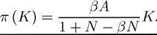
Compare this expression to that in Part 2. What is the effect of an increase in N? Provide in intuition for this.

(5) Show that if βA > 1 > βA∕ (1 + N - βN), than the single-person decision problem would involve growth over time, while the MPE would involve the resources shrinking over time.

(6) Next show that in this game there always exists subgame perfect equilibria that implements the single-person solution for any value of β > 0. Explain this result.

(7) Now suppose that βA = 1 and again focus on MPE. Suppose that the game starts with capital stock K (0) and consider following discontinuous Markovian strategy profile:

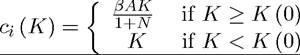
Show that when all players other than i' pursue this strategy, it is a best response for player i' to play this strategy as well, and along the equilibrium path, the single­person solution is implemented. Carefully provide an intuition for this result. Show that the same result cannot be obtained whenWhy not?