CHAPTER B Review of Ordinary Differential Equations
In this chapter, I give a very brief overview of some basic results on differential equations and also include a few results on difference equations. I limit myself to results that are useful for the material covered in the body of the text.
In particular, I provide the background for the major theorems on stability, Theorems 2.2, 2.3, 2.4, 2.5, 7.18, and 7.19, which were presented and then extensively used in the text. I will also provide some basic theorems on existence, uniqueness and continuity of solutions to differential equations. Most of the material here can be found in Simon and Blume (1994) or in basic differential equation textbooks, such as Boyce and DiPrima (1977). Luenberger (1979) is an excellent reference, since it gives a symmetric treatment of differential and difference equations. The results on existence, uniqueness and continuity of solutions can be found in more advanced books, such as Walter (1991). Before presenting the results on differential equations, I also provide a brief overview of eigenvalues and eigenvectors, and some basic results on integrals. Throughout, I continue to assume basic familiarity with matrix algebra and calculus.B. 1. Review of Eigenvalues and Eigenvectors
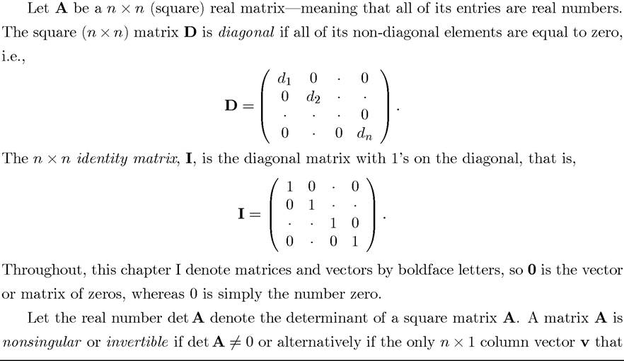
is a solution to the equation
is the zero vector v = (00). If A is invertible, then there exists A-1 such that
Conversely, if there exists a nonzero solution v or if det A =0, then A is singular and does not have an inverse.
result will be used in the proof of Theorem B.5 below and is more generally useful in deriving explicit solutions to systems of linear differential and difference equations.
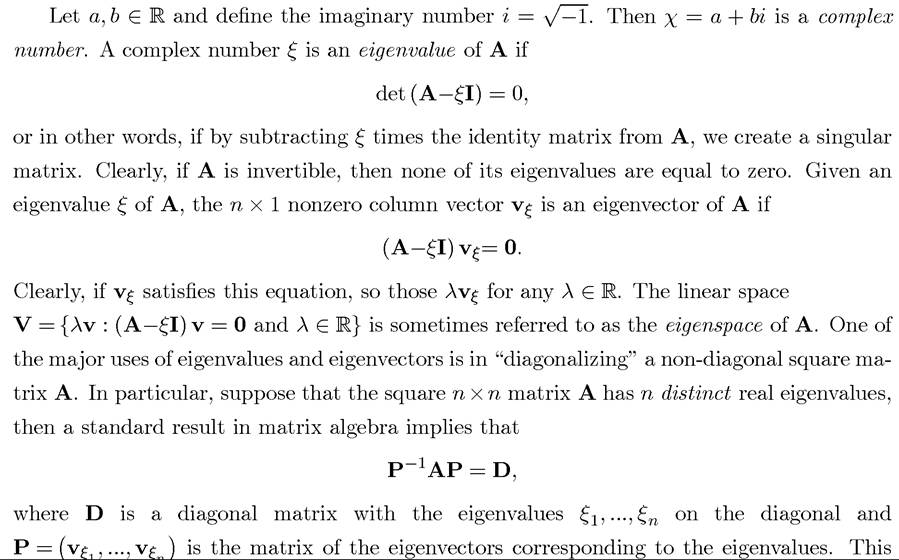
As suggested above, even though all of the entries of A are real, its eigenvalues can be complex numbers. Moreover, we may expect that a n ? n matrix A should have n eigenvalues, since det (A-ξI) = 0 is a polynomial of degree n. However, some of these may be repeated eigenvalues (corresponding to repeated roots to the polynomial). Both of these possibilities create a range of difficulties in diagonalizing the matrix A. These difficulties are discussed in most linear algebra, matrix algebra, and differential equations textbooks, and will not be discussed in detail here.
B. 2. Some Basic Results on Integrals
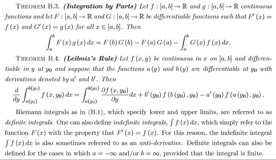
Before proceeding to differential equations, it is useful to review some basic results on integrals. Throughout this section, I will focus on Riemann integrals. In particular, let f : R → R be a continuous function. Then the Riemann integral of f between a and b > a, 1162
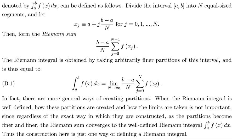
The assumption that f is continuous is not necessary for the Riemann integral to be well-defined (for example, the Riemann integral can be defined for monotone discontinuous functions). But for many functions the Riemann integral is not well-defined. For this reason, it is often more convenient to work with more general integrals, such as the Lebesgue integral. Although I made some references to Lebesgue integrals in the text, here I focus exclusively on Riemann integrals to simplify the discussion. When a function f has a well-defined Riemann integral over the interval [a, b], it is said to be Riemann integrable over [a, b].
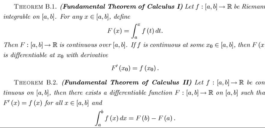
The following four basic results are useful for our analysis. The proofs can be found in standard real analysis or calculus textbooks, and are not repeated here.
n
)
t
1163
B.
3. Linear Differential Equations
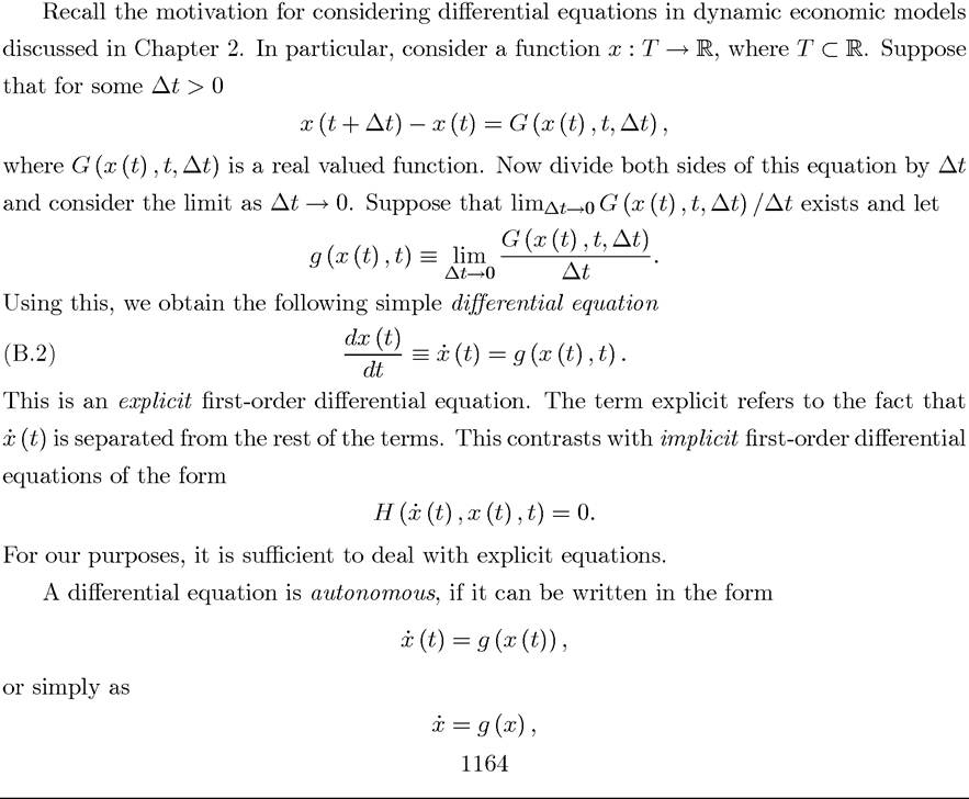
meaning that time is not a separate argument. Alternatively, if it cannot be written this way, it is a nonautonomous equation. In addition to first-order differential equations, we can consider, second order or nth order equations, for example,
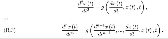
I will focus on first-order equations, since higher-order equations can always be transformed into a system of first-order equations (see Exercise B.2).
The most common form of differential equation is the so-called initial value problem. In this case, a differential equation as in (B.2) is specified together with an initial condition x (0) = xo. We saw many examples of such initial value problems in the text. However, many important problems in economics are not initial value problems, since the boundary
is called the particular solution.
Let us now first look at linear first-order equations. This is a good starting point both because such equations are commonly encountered in economics and they have simple solutions. A linear first-order differential equation takes a general form

In addition, if b (t) = 0, this is referred to as a homogeneous equation and if a (t) = a and b (t) = b, then it is an equation with constant coefficients.
Let us start with the simplest case, which is a homogeneous linear equation with constant coefficients, i.e.,

A solution to this equation is straightforward to obtain. One can simply guess the solution and then verify that the solution satisfies the differential equation (B.5).
Or one can divide both sides by x (t), integrate with respect to t and recall that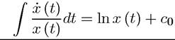
and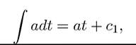
where co and ci are constants of integration. Now taking exponents on both sides, the solution to (B.5) is obtained as
(B.6)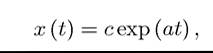
where c is a constant of integration combining co and ci (in fact, c = exp (ci — co)). Differentiating this equation, one easily obtains (B.5) and verifies that (B.6) is indeed a solution to (B.5). If (B.5) is specified as an initial value problem, then we also have a boundary condition, which, without loss of any generality, can be specified at t = 0 as x (0) = xo. This boundary condition pins down the unique value of the constant of integration. In particular, since exp (a ? 0) = 1, c = xo.
Next consider a slightly more general equation, homogeneous but not with constant coefficients, that is,
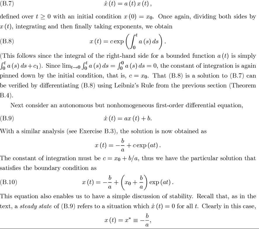
is the unique steady state. Inspection of (B.10) immediately shows that x (t) will approach the steady-state value x* as t increases if a < 0 and it will diverge away from it if a > 0. This is naturally what we would expect from Theorem 2.4, which states that the steady state is asymptotically stable if a < 0.
Finally, let us consider the most general case of the first-order linear differential equation, that given in (B.4). Once again, with an analysis similar to that in Exercise B.3, we obtain the general solution to (B.4) as
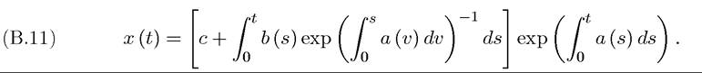
Differentiation using Leibniz’s Rule verifies that (B.11) provides the solution to (B.4) (see Exercise B.4). A similar analysis to that above, allows us to derive the constant of integration from the initial value x (0) = xo as c = xo.
Notice, however, that in this case there is no steady-state value of x* for which in (B.4), since
 implies x (t) = —b (t) /a (t), which is generally not a constant.
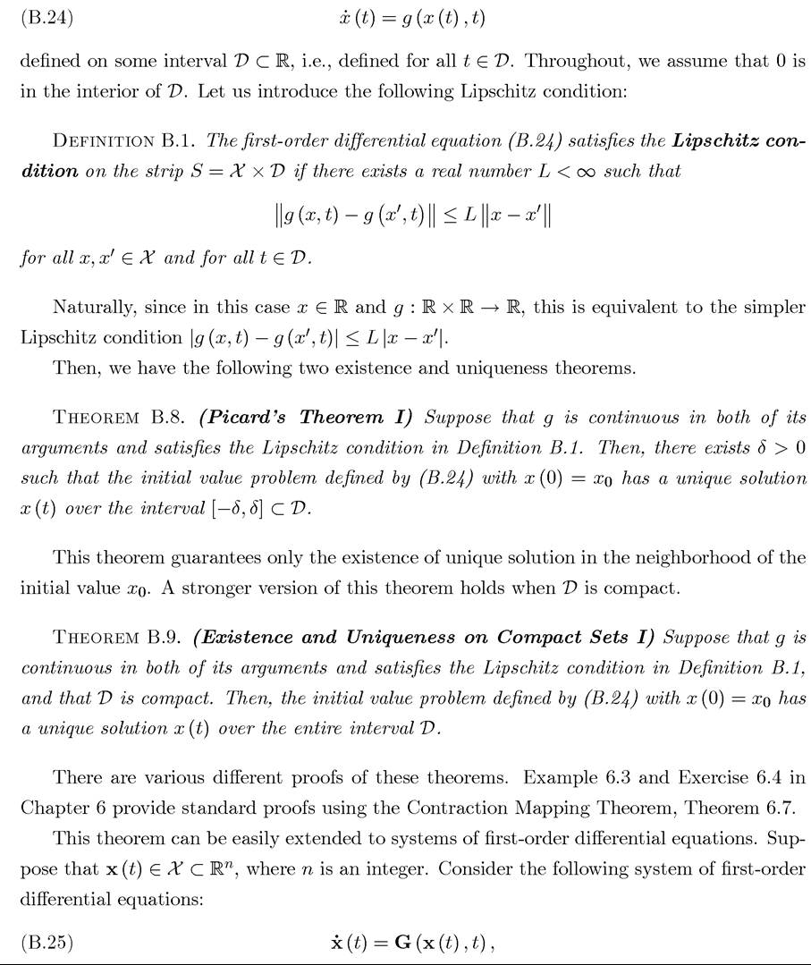
A byproduct of this brief discussion is that we have also established the existence of unique solutions to linear differential equations (since we have provided explicit solutions). Thus linear differential equations (formulated as initial value problems) always have a solution. Moreover, the solution is unique. This is a special case of Theorem B.8 below.
The results on the existence of solutions and explicit characterization of solutions for linear first-order differential equations can be extended to systems of differential equations. The general result here is provided in Theorem B.6. However, before presenting this more general result, it is useful to consider the following simpler system of first-order differential equations with constant coefficients:

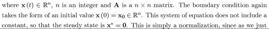
saw, a nonhomogeneous differential equation with constant coefficients can be transformed into a homogeneous one by a simple change of variables. This system of differential equations always has a unique solution (this follows from Theorem B.6 for from Theorem B.10, see Exercise B.5). However, when A has distinct real eigenvalues, the solution to (B.12) takes a particularly simple form. This case is presented in the next result.
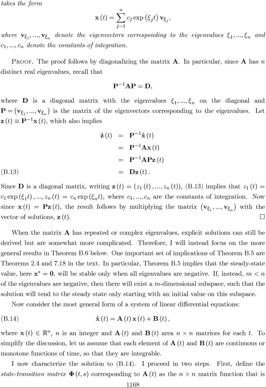
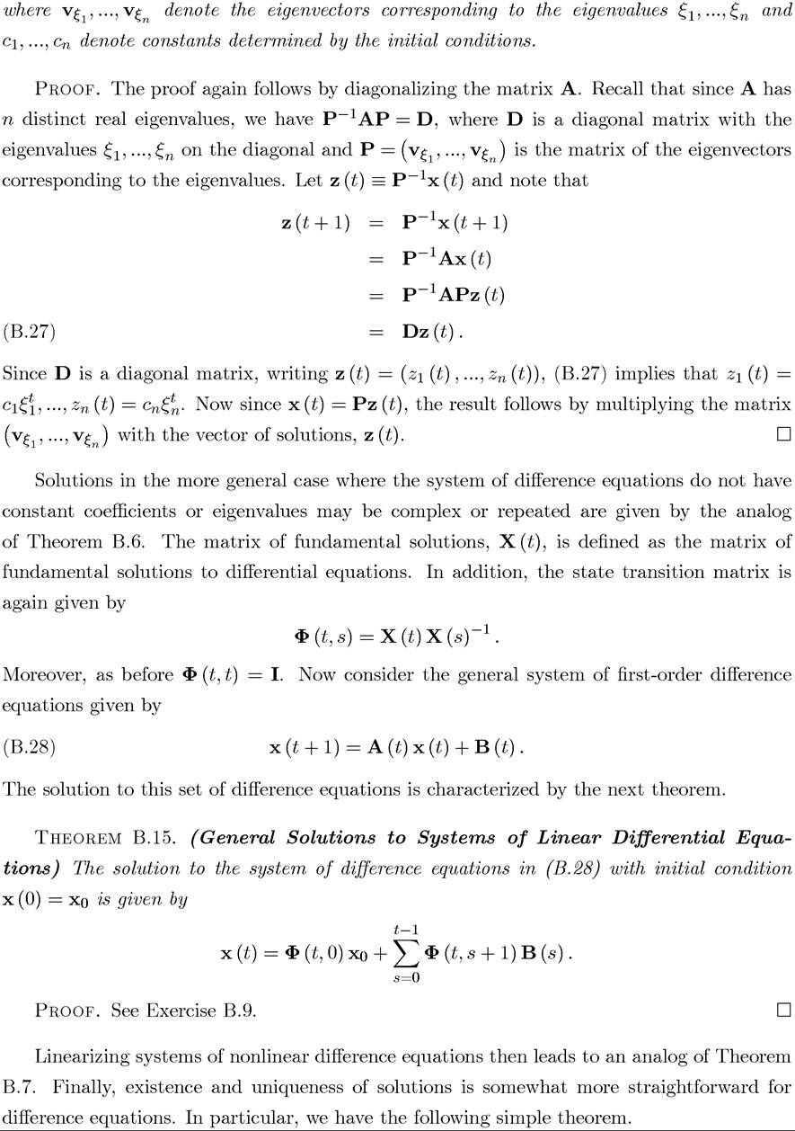
Theorem B.5. (Solution to Systems of Linear Differential Equations with Constant Coefficients) Suppose that A has n distinct real eigenvalues ξ 1,...,ξn, then the unique solution to the system of linear differential equations (B.12) with the initial value x (0) = xo 1167
The state-transition matrix is useful because it enables us to express the solutions to homogeneous systems and then derive the solutions to (B.14) from the solutions to the corresponding homogeneous systems.
In particular, if x (t) is a solution to the homogeneous system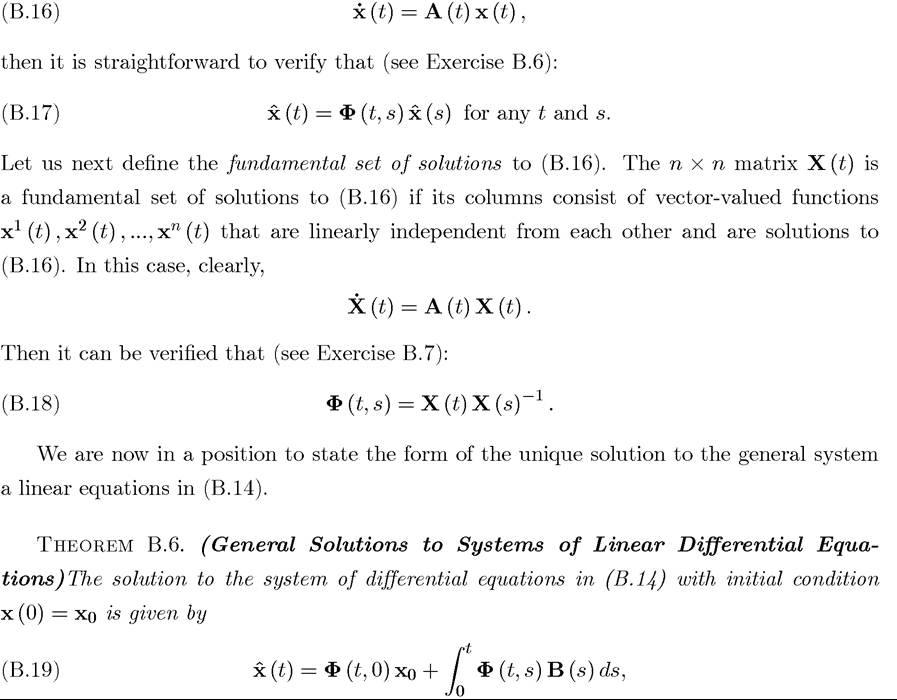
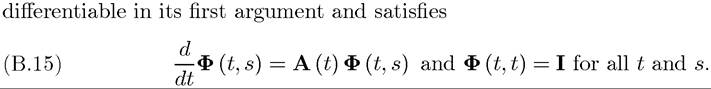
where Φ (t, s) is the state transition matrix corresponding to A (t).
Proof. We only need to verify that x(t) given in (B.19) is a solution to (B.14). Let us simplify notation of time derivatives by writing this as x (t). Differentiating (B.19) with respect to time and using Leibniz’s Rule (Theorem B.4), we obtain
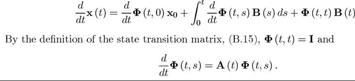
Therefore,
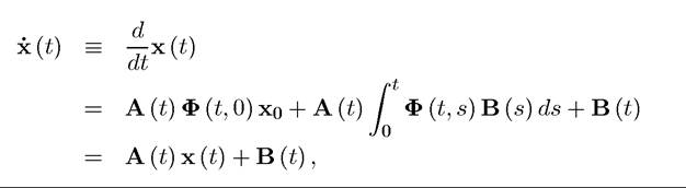
completing the verification that (B.19) satisfies (B.14) with initial condition x (0) = xo. ?
B.4. Stability for Nonlinear Differential Equations
Systems of nonlinear differential equations can be analyzed in the neighborhood of the steady state by using Taylor’s Theorem (Theorem A.21). In particular, consider the system of nonlinear autonomous differential equations 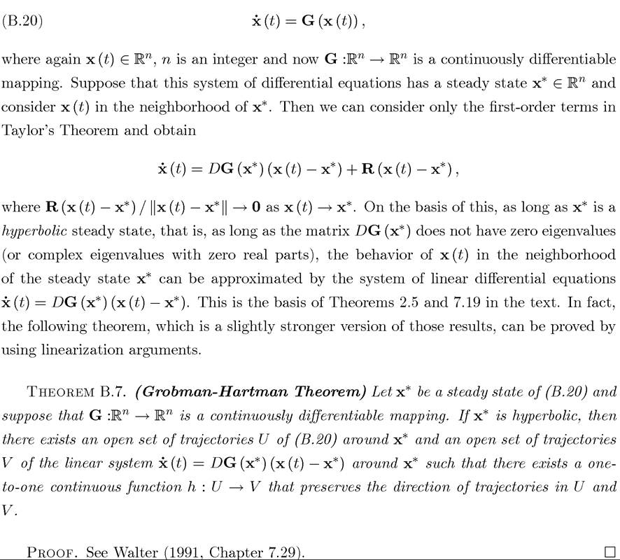
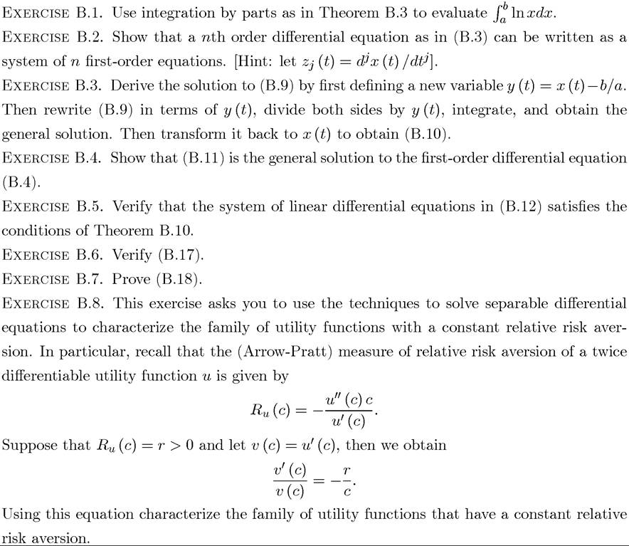
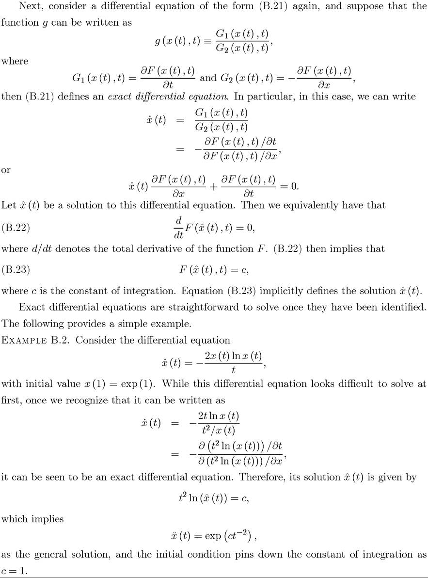
B. 5. Separable and Exact Differential Equations
We cannot obtain explicit solutions to nonlinear differential equations in general (though existence of solutions can be guaranteed under some conditions as shown in the next section). Nevertheless, two important special classes of differential equations, separable and exact differential equations, often enable us to derive explicit solutions. I start with separable differential equations. A differential equation
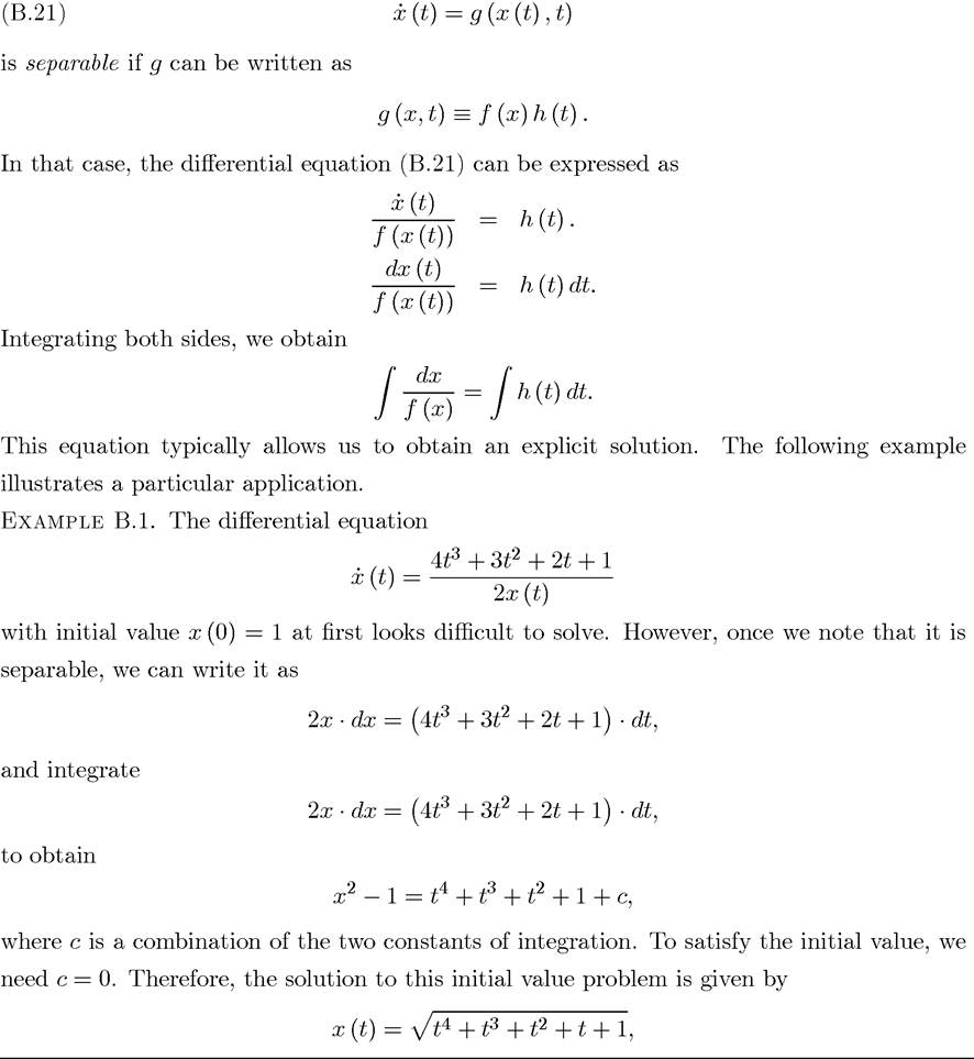
where the negative root to the quadratic is eliminated because it does not satisfied the initial value x (0) = 1.
Another example, which is more relevant for economic applications, is given in Exercise
B.8.
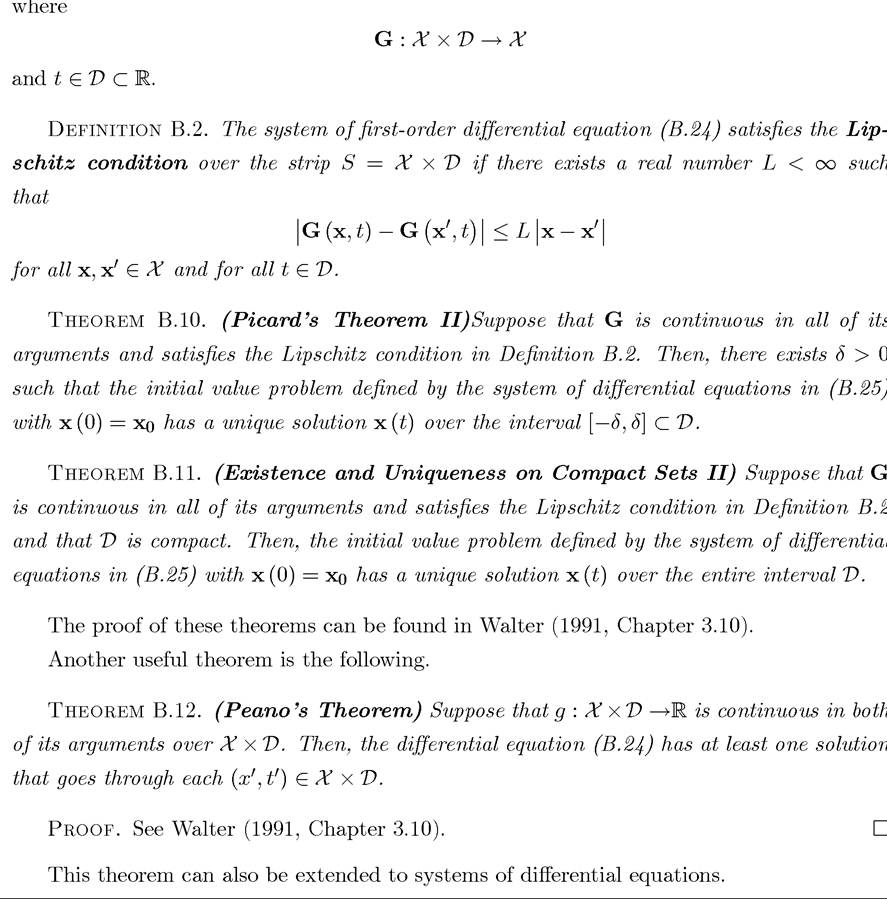
B. 6. Existence and Uniqueness of Solutions
Initial value problems generally enable us to establish the existence and uniqueness of solutions under relatively weak conditions. In fact, there are many related existence theorems. I will state the most basic existence theorem here, which extends the original theorem by Picard. Consider a first-order differential equation
1173
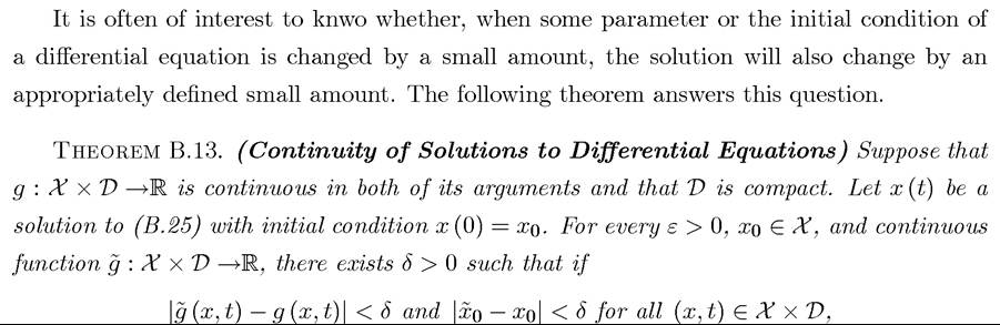
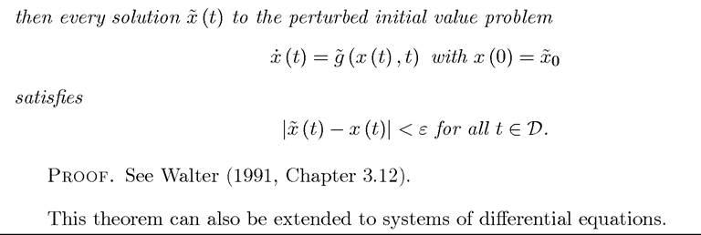
B.7. Continuity of Solutions
1174
I
I
l
)
l
l
I
 ?
?
B.8. Difference Equations
Solutions to difference equations have many features that are common with the solutions to differential equations. For example, the simple first-order difference equation
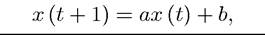
has a solution similar to the first-order linear differential equation with constant coefficients.
In particular, if we specify the initial condition x (0) = xo, then successive substitutions yield
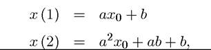
and so on. Therefore, the general solution to this equation is 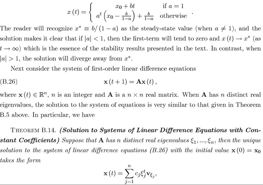
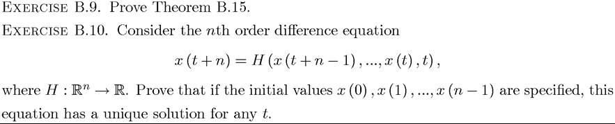
B.9. Exercises