CHAPTER A Odds and Ends in Real Analysis and Applications to Optimization

This chapter is included as a review of some basic material from real analysis. Its main purpose is to make the book self-contained and also include explicit statements of some of the theorems that are appealed to in the text.

It should be emphasized that the material here is not a substitute for a basic “Mathematics for Economists” type review or textbook. An excellent book of this sort is Simon and Blume (1994), and I will presume that the reader is familiar with most of the material in this or a similar book. In particular, I assume that the reader is comfortable with linear algebra, functions, relations, set theoretic language, calculus of multiple variables, and basic proof techniques.

To gain a deeper understanding and appreciation of the material here, the reader is encouraged to consult one of many excellent books on real analysis, functional analysis, and general topology. Some of the material here is simply a review of introductory real analysis more or less at the level of the classic books by Rudin (1976) or Apostol (1974). Some of the material, particularly those concerning topology and infinite-dimensional analysis, are more advanced and can be found in Conway (1990), Kelley (1955), Kolmogorov and Fomin (1970), Royden (1994), and Aliprantis and Border (1999).

A. 1. Distances and Metric Spaces

Of special importance for our purposes here are two types of spaces: (1) finite-dimensional Euclidean spaces, which I will denote bywhere K is an integer; (2) infinite­

dimensional spaces, such as spaces of sequences or spaces of functions, which feature in discrete-time and continuous-time dynamic optimization problems. For our purposes, the most useful sets are those that are equipped with a metric, so that they can be treated as a metric space. Metric spaces play a major role in the analysis of dynamic programming problems in Chapters 6 and 16.

A nonempty set X equipped with a metric d constitutes a metric space (X,d).

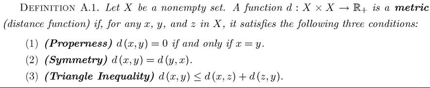
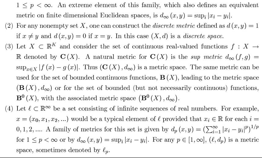
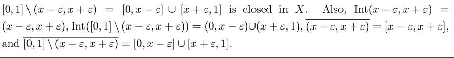
The same set can be equipped with different metrics. This will sometimes facilitate the analysis, but in many cases, different metrics give equivalent results. In this case, we say that two metrics are equivalent, and the definition for this is given below in Definition A.4 (but I am mentioning this here, since I will refer to equivalent metrics in the next example). EXAMPLE A.1. The following are examples of metric spaces. In each case, properness and symmetry are easy to verify, but verifying that the triangle inequality holds requires some work (see Exercise A.2).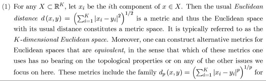

¹Throughout this chapter, I will simplified the notation and use “=” for definitions instead of

Metric spaces are particularly useful because they enable us to define neighborhoods and open sets, which are the building blocks of mathematical analysis and essential elements for our investigation of optimization problems.

Definition A.2. Let (X, d) be a metric space and ε > 0 be scalar. Then for any x ∈ X, is the ε-neighborhood of x.

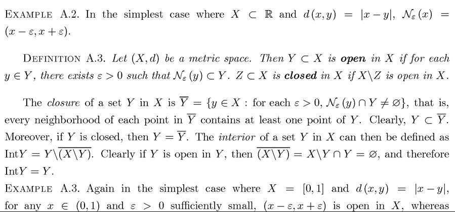
FACT A.1. Let (X,d) be a metric space. X and 0 are both open and closed sets.

The importance of the following theorem will become clear once we turn to the somewhat more abstract topological characterization of closed and open sets. Let A be a set of real numbers (for example, N). Thenis a collection of sets. If A is countable [finite], then {X_α}_α∈A is a countable [finite] collection of sets, but it can also be an arbitrary collection of sets. In referring to collections of sets, I will take it as implicit that A is a set of real numbers. Let us also use X£ to denote the complement of X_α in X, i.e.,

Theorem A.1. (Properties of Open and Closed Sets) Let (X, d) be a metric space andbe a collection of sets with.

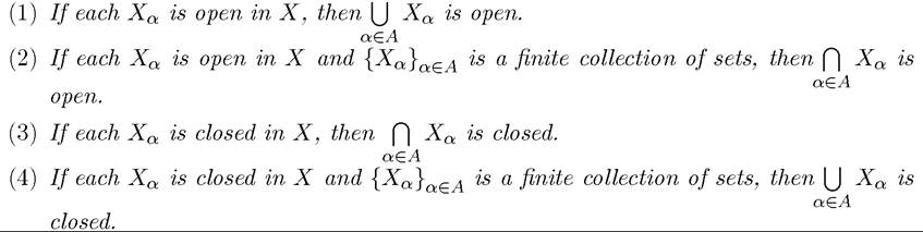
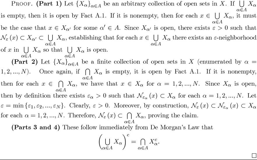
The restriction to finite collections is important in Part 2 of Theorem A.1.

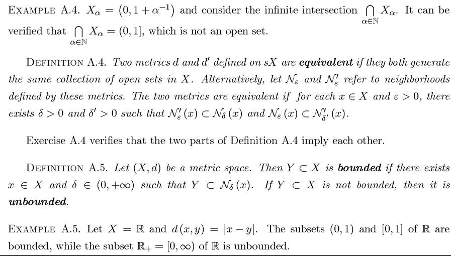
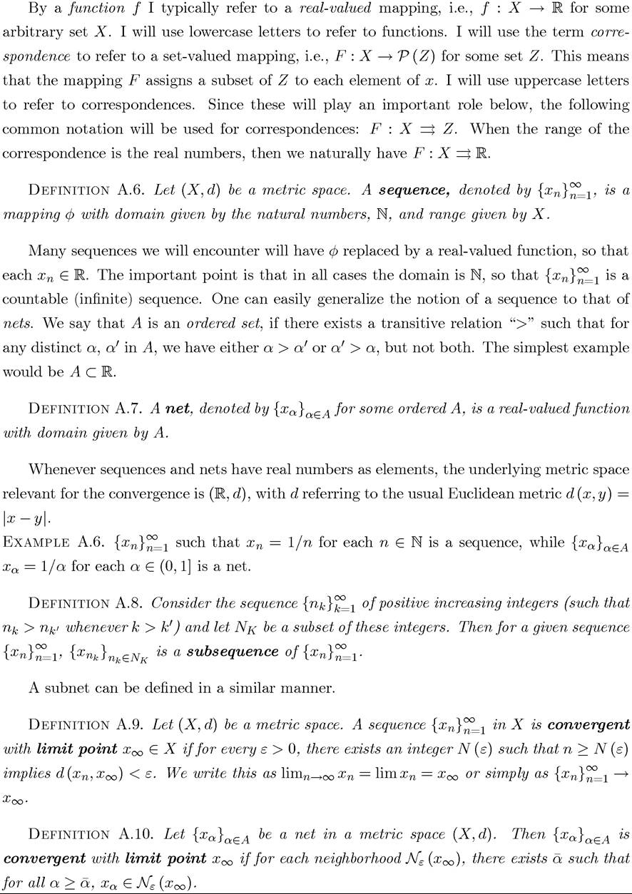
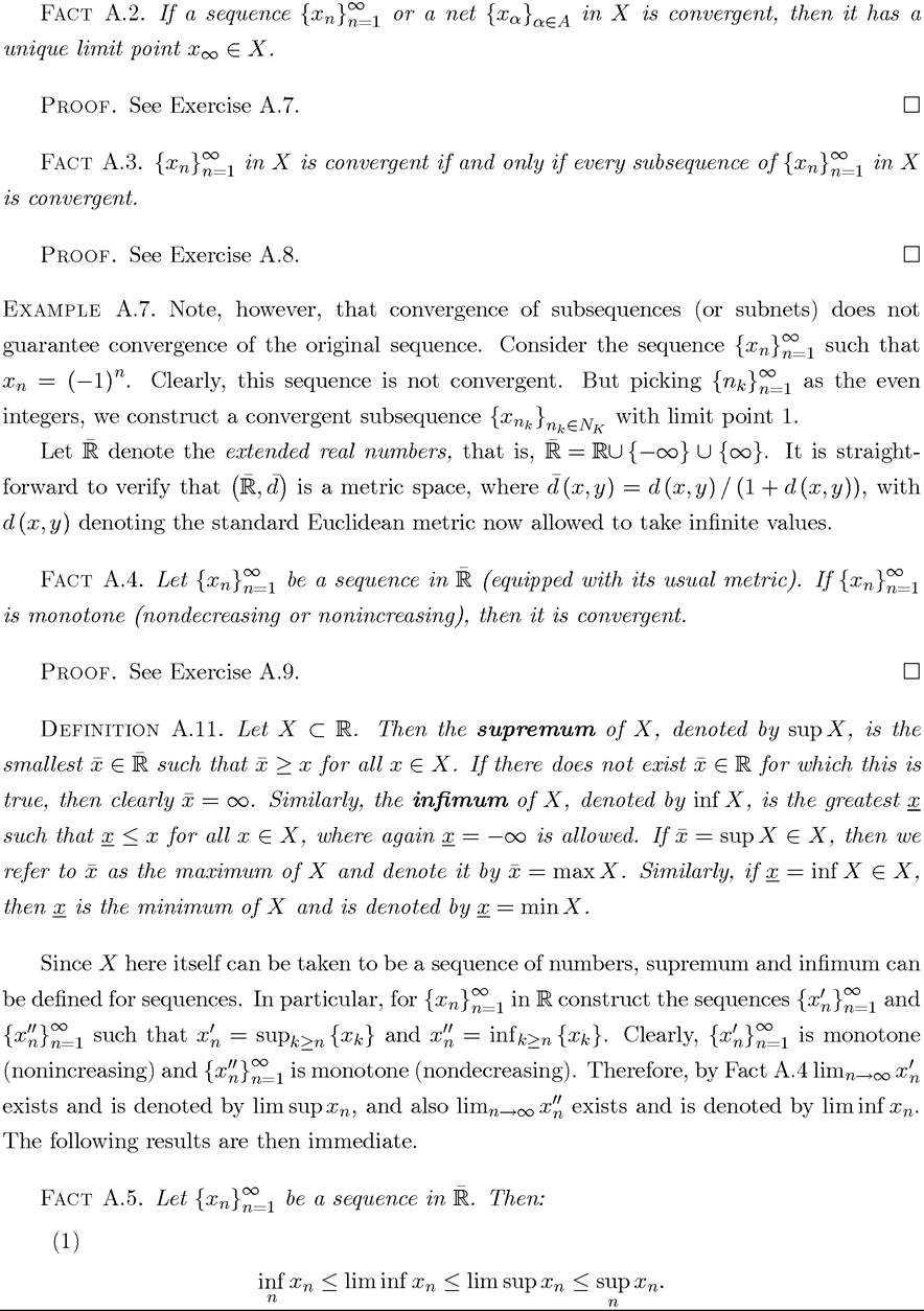
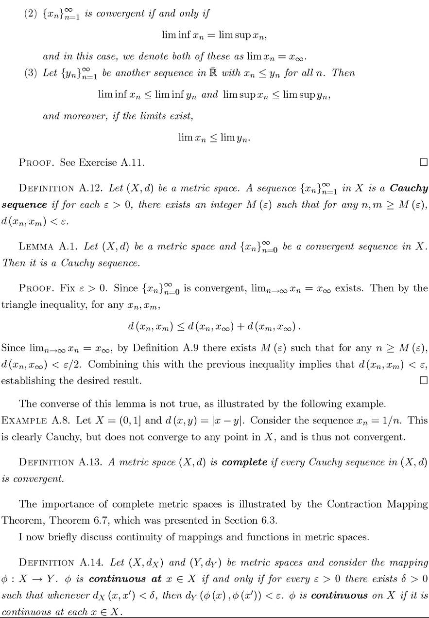
A. 2. Mappings, Functions, Sequences, and Continuity

1121

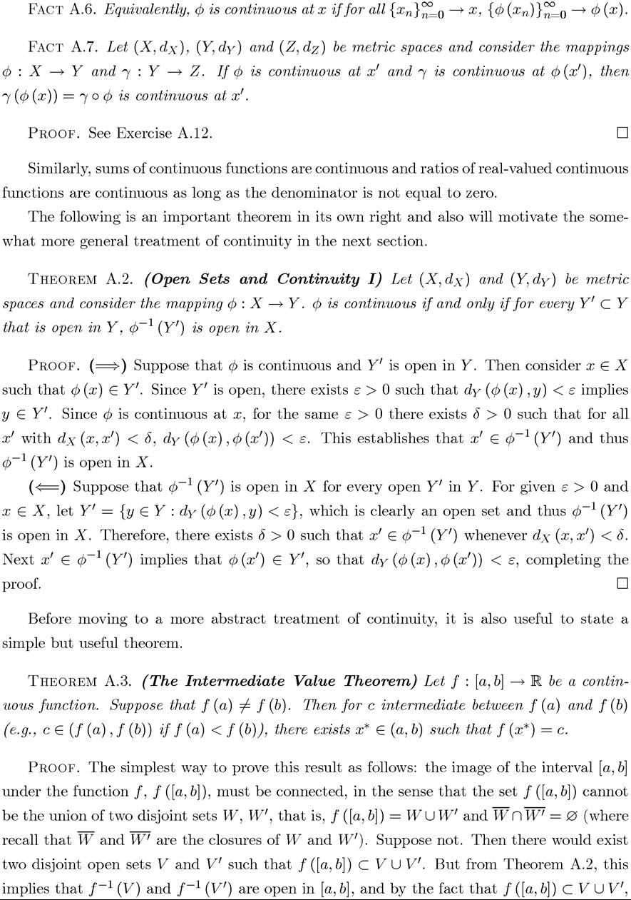
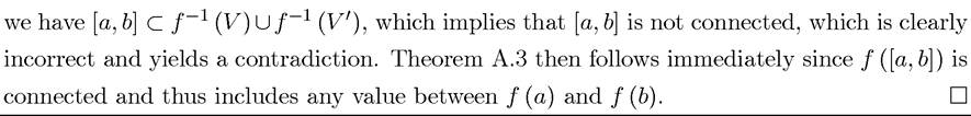
The Intermediate Value Theorem is, in many ways, the simplest “fixed point theorem” that economists can use in some applications (see Theorems A.16 and A.17 below for more general fixed point theorems). Fixed point theorems require a mapping φ : X → X to have a point x* ∈ X such that x* = φ (x*). The usefulness of this construction stems from the fact that many equilibrium problems can be formulated as fixed point problems. It is also clear that a fixed point is nothing but a “zero” of a slightly different mapping. In particular, define φ (x) = φ (x) — x. Then a fixed point of φ corresponds to a zero of φ. Perhaps the most useful application of the Intermediate Value Theorem is for the case in which f (a) < 0 and f (b) > 0 (or f (a) > 0 and f (b) < 0). In this case, the theorem states that the continuous function f has a “zero” over the interval [a, b], that is, some value x* ∈ (a, b) such that f (x*) = 0. This motivates my description of the Intermediate Value Theorem as the “simplest fixed point theorem”.

A. 3. A Minimal Amount of Topology: Continuity and Compactness

Theorem A.2 implies that only the structure of open sets are relevant for thinking about continuity of mappings.

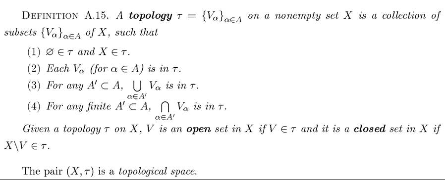
The parallel between this definition and the properties of unions and intersections of open sets given in Theorem A.1 is obvious. Sometimes it is convenient to describe a topology not 1126

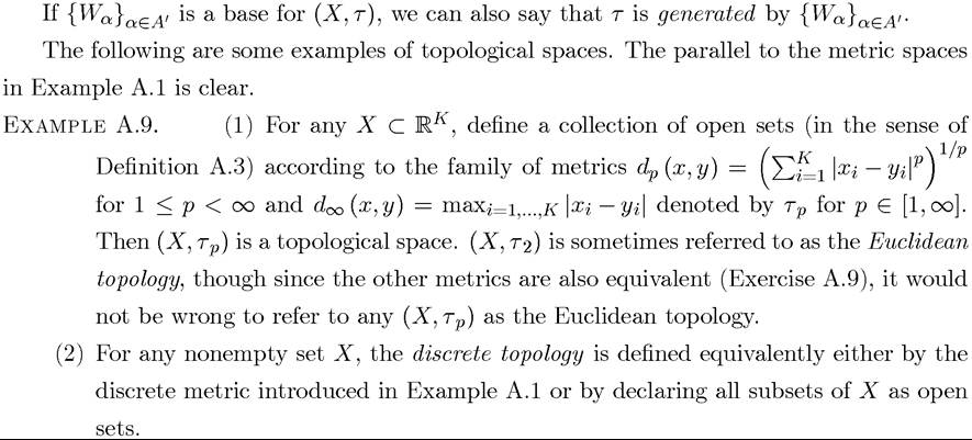
by all of the open sets, but in a more economical fashion. Two convenient ways of doing this are as follows. First, a topological space can be derived from a metric space. In particular, since a topological space (X, τ) is defined by a collection of open sets and a metric space (X, d) defines the collection of open sets in the space X, it also immediately defines a topological space with the topology induced by the metric d. Second, a topological space can be described by a smaller collection of sets (instead of the collection of open sets). This leads us to the concept of a base for a topology.

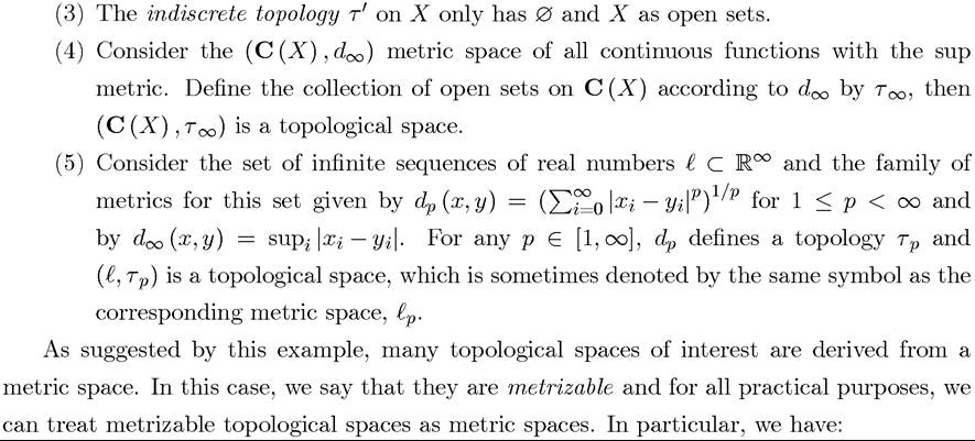
Definition A.17. A topological space (X,τ) is metrizable if there exists a metric d on X such that if V ∈ τ, then V is open in the metric space (X, d) (according to Definition A.3).

FACT A.8. If a topological space (X,τ) is metrizable with some metric d, then it has all the topological properties of the metric space (X, d).

Proof. This follows immediately from the fact that (X, τ) and (X, d) have the same open sets.

The preceding definition and fact are provided, because metric spaces are easier to work with in practice than topological spaces. Nevertheless, sometimes (as with the product topol­ogy introduced in the next section), it may be more convenient to work with more general topological spaces. One disadvantage of general topological spaces is that they do not have all of the nice properties of metric spaces. However, this will not be an issue for the prop­erties of topological spaces that are related to continuity and compactness, which will focus on here. Nevertheless, it is useful to note that a particularly relevant property of general topological spaces is the Hausdorff property, which requires that any distinct points x and

Returning to general topological spaces, the notions of convergence of sequences, subse­quences, nets and subnets can be stated for general topological spaces. Here I will only give the definitions for convergence of sequences and nets (those for subsequences and subnets are defined very similarly).

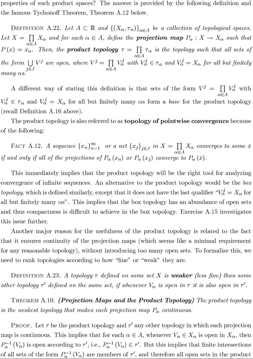
A.4. The Product Topology

One of the main reasons for introducing topological spaces rather than simply working with metric spaces is to introduce the product topology. The product topology is particularly useful when dealing with infinite-dimensional optimization problems, since we can represent the space of sequences, I, as the infinite product of R, i.e., as R∞. What are the topological

²In fact, there are many theorems that go under the name of “Weierstrass’s Theorem,” including on uni­form continuity of a family of functions and approximation of continuous functions by polynomials. However, since these theorems are not used commonly in economic applications, there should be little confusion in referring to Theorem A.9 as Weierstrass’s Theorem.

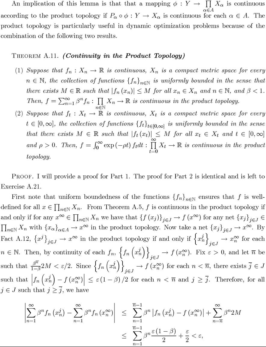
topology τ belong to τ'. Thus τ' must be finer than τ and establishes that the product topology is the weakest topology in which each projection map is continuous. ?

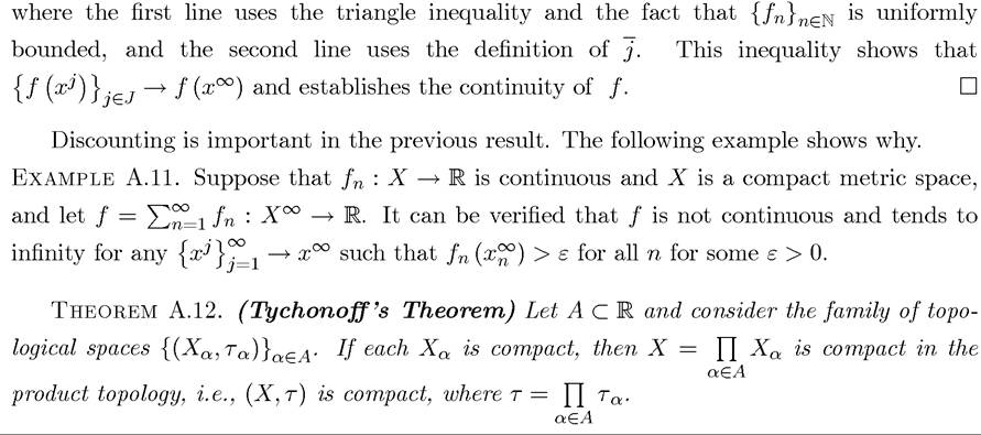
The proof of this theorem is somewhat involved, and can be found in Kelley (1955) or Royden (1994).

Combined with Theorem A.11, this theorem implies that problems involving the maxi­mization of discounted utility in standard dynamic economic environments has a continuous objective function in the product topology. We can then appeal to Tychonoff's Theorem to make sure that the relevant constraint set is compact (again in the product topology). This combination then enables us to apply Weierstrass's Theorem, Theorem A.9, to show the existence of solutions. The reader will recall that we have used this technique in Chapters 6, 7, and 16.

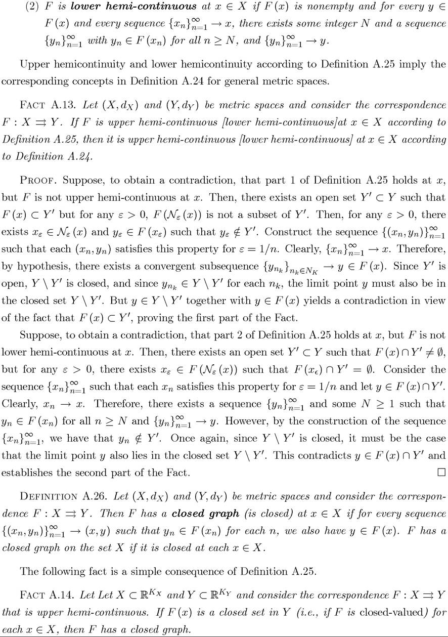
A.5. Correspondences and Berge’s Maximum Theorem

In this section, I state one of the most important theorems in economic analysis, Berge's Maximum Theorem. This theorem is not only essential for dynamic optimization, but it plays a major role in general equilibrium theory, game theory, little economy,producer theory, public finance and industrial organization. In fact, it is hard to imagine any area of economics where it does not play a major role. Despite its enormous importance, this theorem is left out of most basic “Mathematics for Economists” courses and textbooks. This motivates my somewhat detailed treatment of it here. The first step for this theorem is to have a brief review of correspondences, which were already mentioned above.

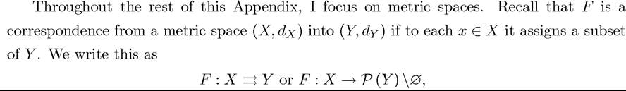
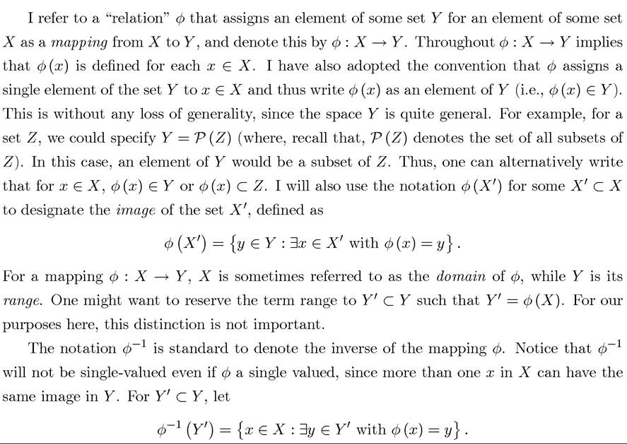
where P (Y) is the power set of Y (and I have subtracted the empty set 0, so that the corre­spondence is not empty valued). We are interested in correspondences for three fundamental 1134

reasons. First, even when a mapping into real numbers is a well behaved function, f : X → R, its inverse f^-1 will typically be set-valued, thus a correspondence. Second, our main interest in most economic problems is with the “arg max” sets defined above, which are the subsets of values in some set X that maximize a function. These will correspond to utility-maximizing consumption, investment or price levels in simple economic problems. Finally, and perhaps most importantly, correspondences will play a key role both as representing economically rele­vant constraints and as a way of expressing the properties of maximizers in Berge’s Maximum Theorem.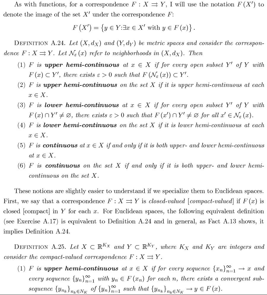

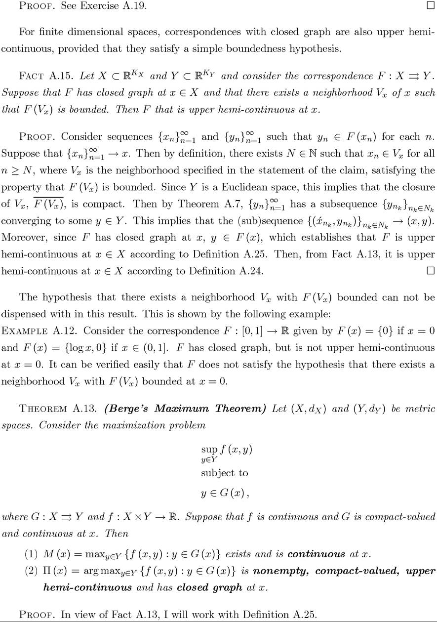
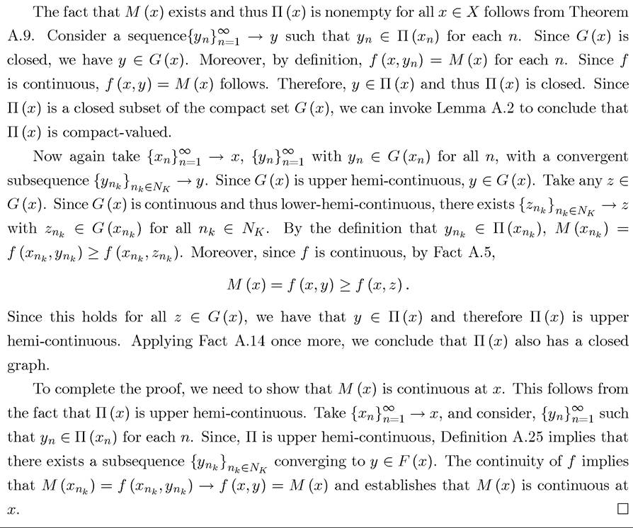
Note that I wrote the maximization problem as sup_y∈_v instead of maxy∈γ. There would have been no loss of generality in using the latter notation, since the theorem establishes that the maximum is attained. Nevertheless, the former might be slightly more appropriate, since when we first consider the problem with do not know whether the maximum is attained or not. Throughout the appendix, I used the “sup” notation, while in the text I typically use the simpler “max” notation.

One difficulty in using Theorem A.13 is that constraint sets do not always define contin­uous correspondences. This is illustrated in Exercise A.18. However, Fact A.16 shows that in some important cases they do in fact define continuous correspondences.

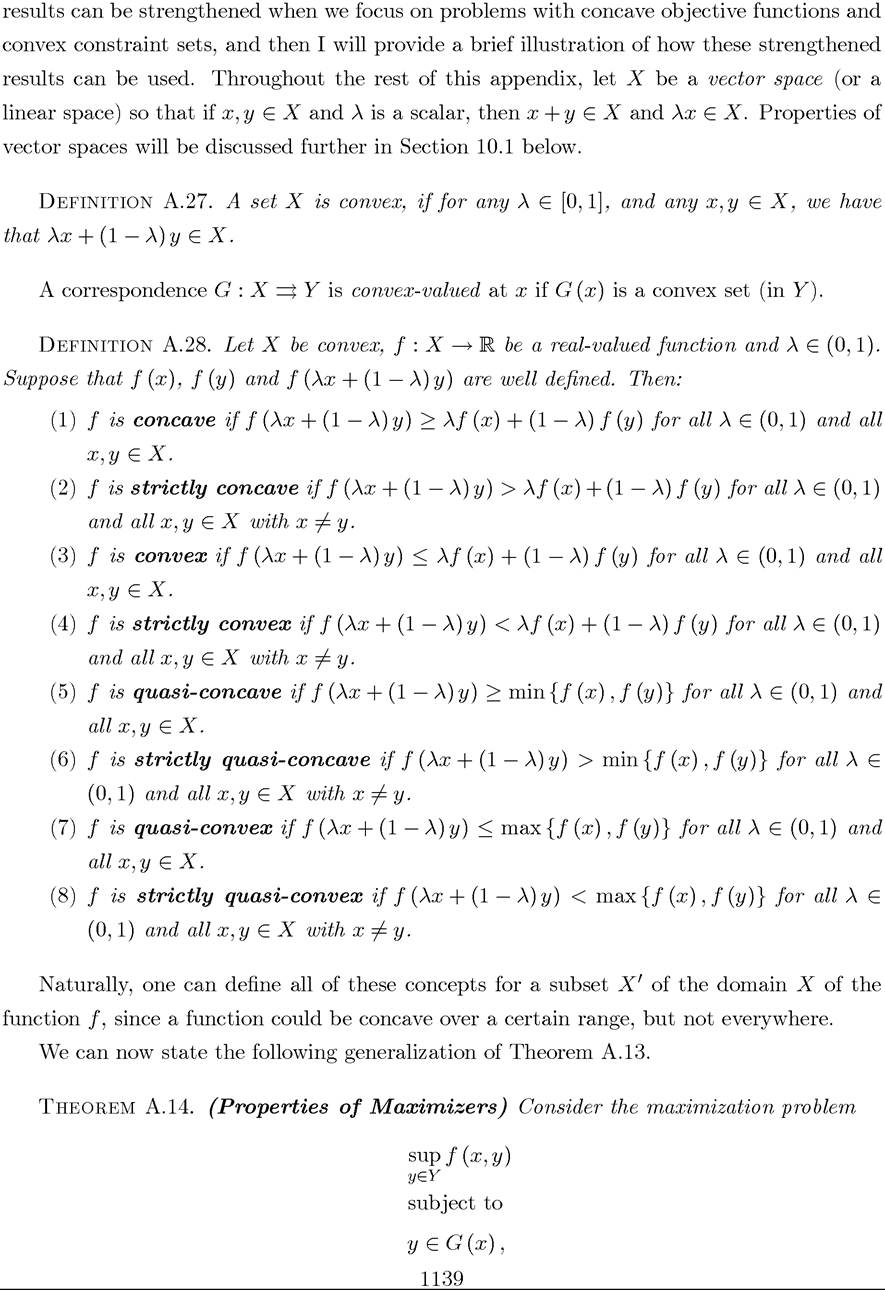
A.6. Convexity, Concavity, Quasi-Concavity and Fixed Points

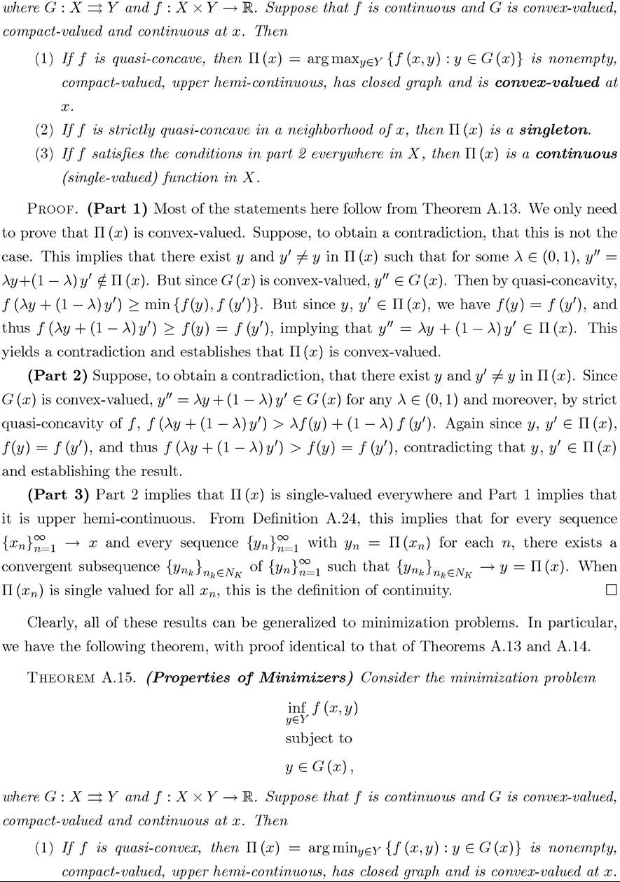
Theorem A.13 shows how we can ensure certain desirable properties of the set of maxi­mizers in a variety of problems arising in economic analysis. However, it is not strong enough to assert uniqueness of maximizers or continuity of the set of maximizers (instead, we have upper hemi-continuity, which is weaker than continuity). In this section, I will show how these 1138

id="Picutre 3371" class="lazyload" data-src="/files/uch_group77/uch_pgroup317/uch_uch7364/image/image3369.jpg">

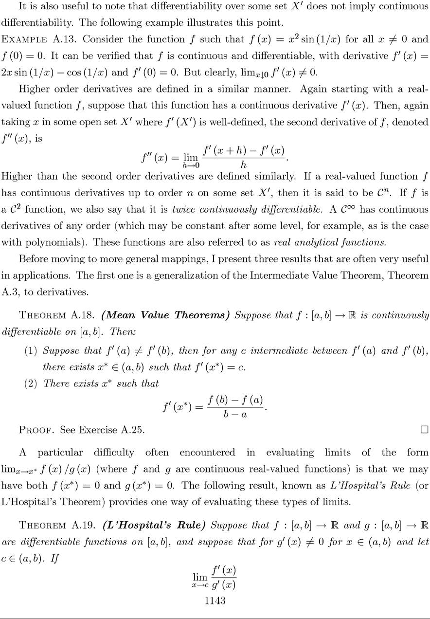
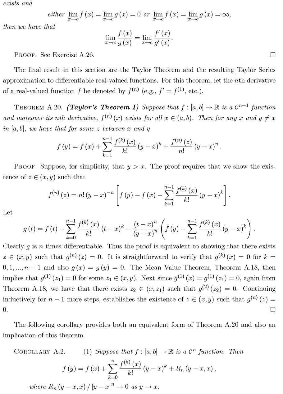
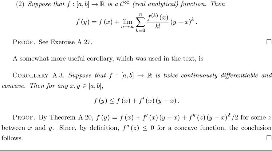
A.7. Differentiation, Taylor Series and the Mean Value Theorem

In this and the next section, I briefly discuss differentiation and some important results related to differentiation that are useful for the analysis in the text. The material in this section should be more familiar, thus I will be somewhat more brief in my treatment. In this section, the focus is on a real-valued function of one variable f : R → R. Functions of several variables and vector-valued functions are discussed in the next section.

The reader will recall that the derivative (function) for f : R → R has a simple definition. Take a point x in an open set X' on which the function f is defined. Then, when it exists, the derivative of f at x is defined by the following limit

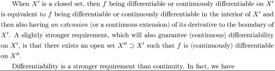
Clearly, the term f (x + h) is well defined for h sufficiently small since x is in the open set X'. Moreover, this limit will exist at point x only if f is continuous at x ∈ X. This is a more general property; differentiability implies continuity (see Fact A.17). Using the elementary properties of limits, expression in (A.1) can be rearranged as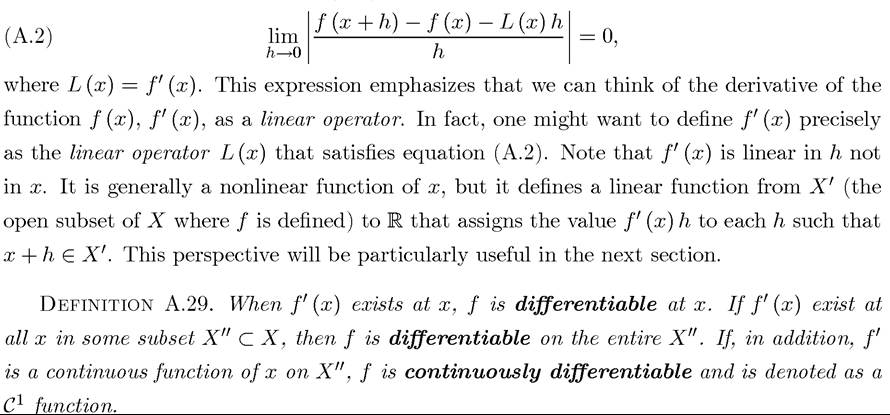

Proof. See Exercise A.24.

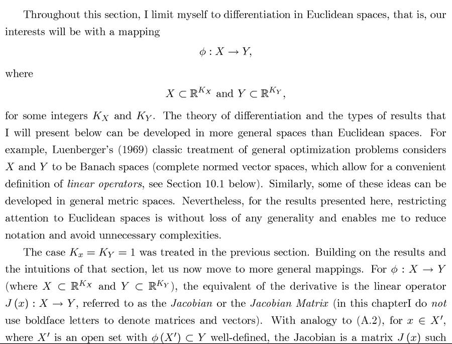
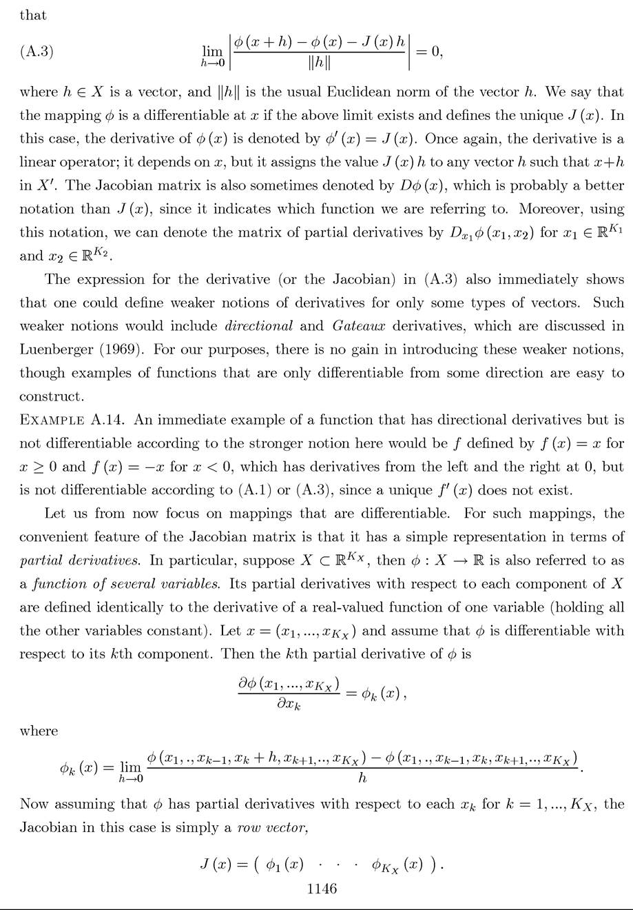
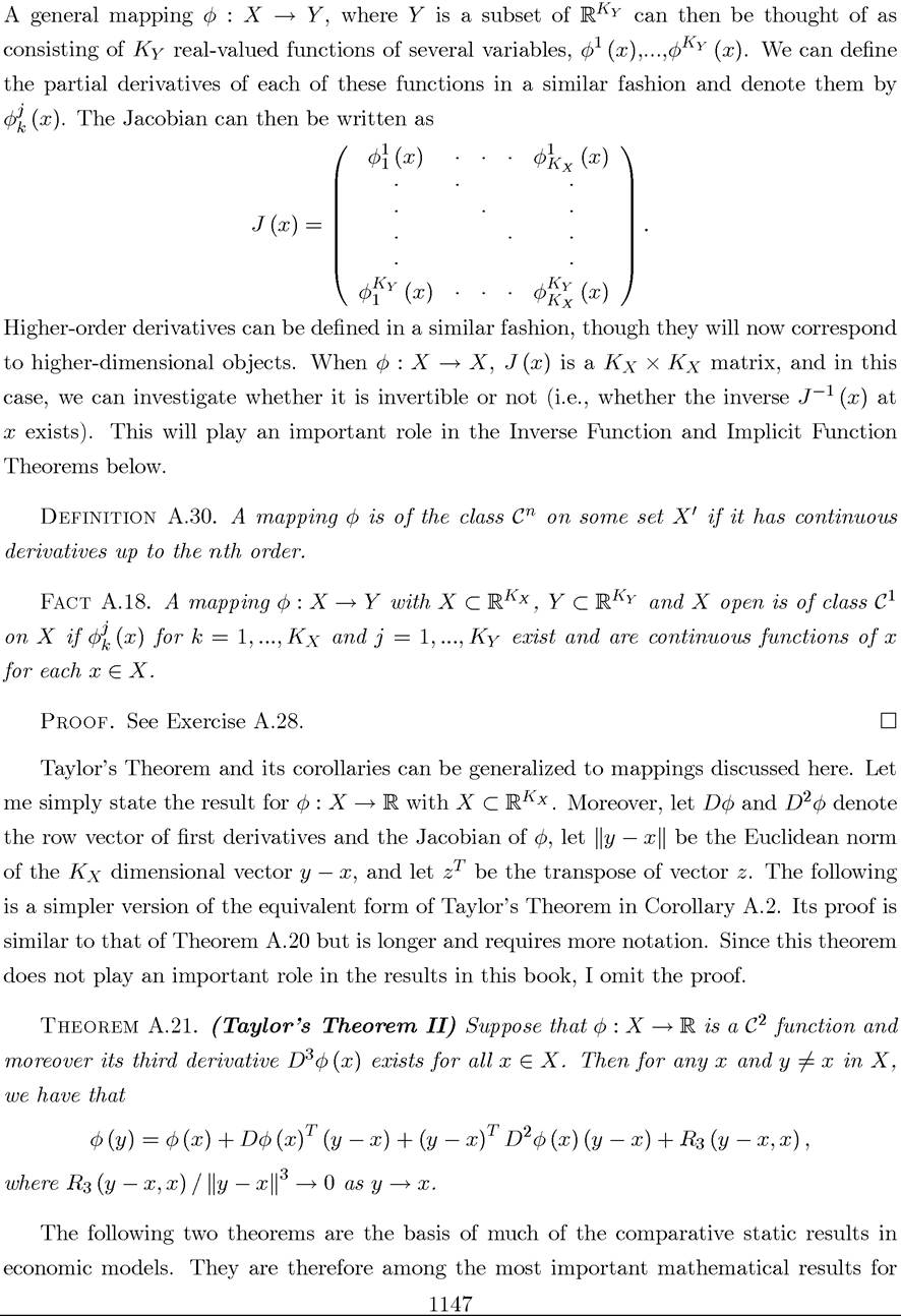
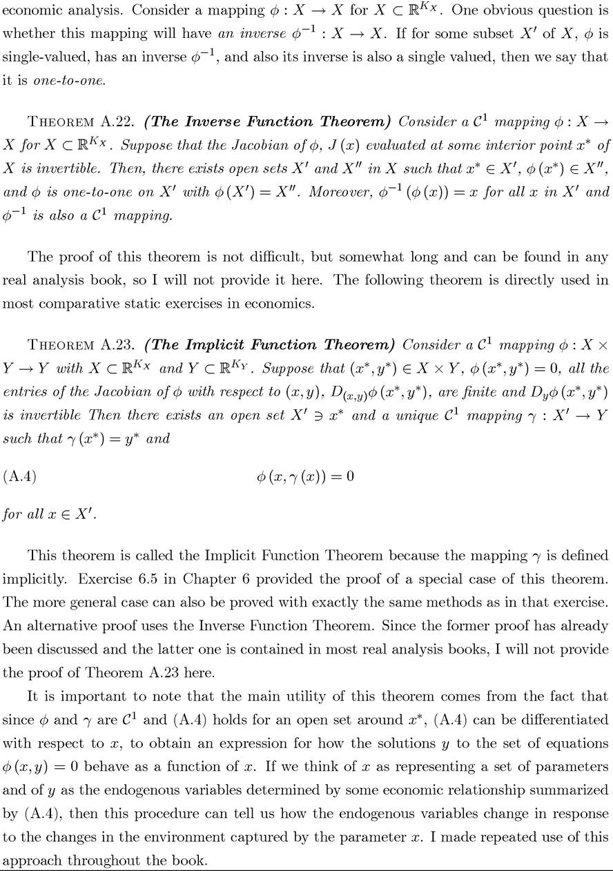
A.8. Functions of Several Variables and the Inverse and Implicit Function Theorems

1145

A.9. Separation Theorems

In this section, I will briefly discuss the separation of convex disjoint sets using linear functionals (or hyperplanes). These results form the basis of the Second Welfare Theorem, provided in Theorem 5.7 in Chapter 5. They also provide the basis of many important results in constrained optimization (see Section A.10).

For this section, we take X be a vector space (linear space). Recall from Section A.6) that this implies: if x,y ∈ X and λ is a scalar, then x + y ∈ X and λx ∈ X. The element of X with the property that x = λx for all scalar λ is denoted by θ. Moreover, we have: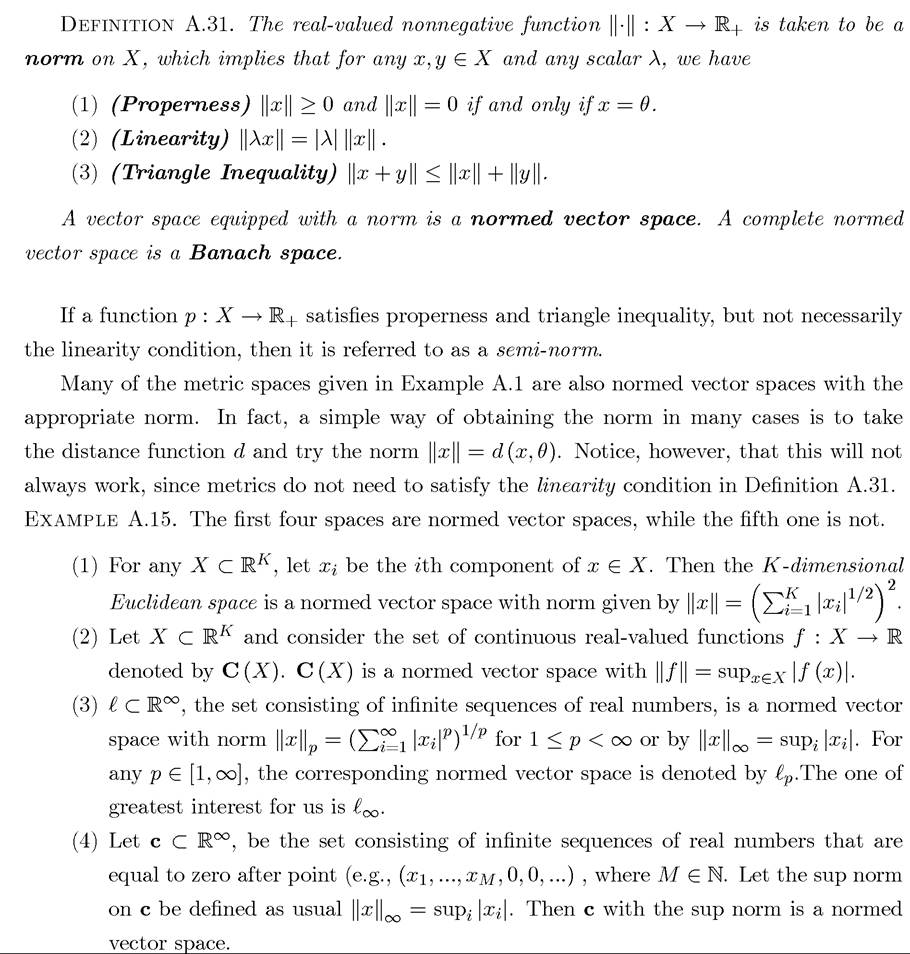

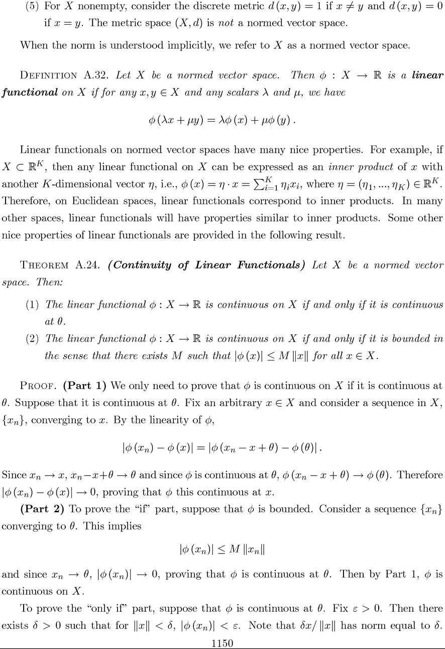
Therefore,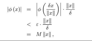

with M = ε∕δ, completing the proof. ?

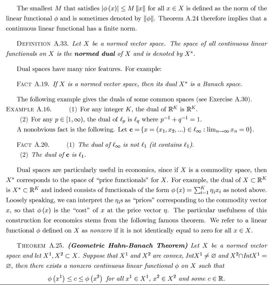
This theorem is a straightforward consequence of the Hahn-Banach Theorem. The Hahn-

Banach Theorem states that if φ is a continuous linear functional on a subspace M of X and 1151

is dominated by a semi-norm p (x), i.e., f (x) ≤ p (x) for all x ∈ M, then there is an extension Φ of φ to the entire X such that Φ is a continuous linear functional on X, Φ (x) = φ (x) for all x ∈ M and Φ (x) ≤ p (x) for all x ∈ X. This theorem therefore establishes that normed vector spaces are “abundant” in linear functionals. More important for our purposes, it also implies Theorem A.25. Since its proof is not particularly useful for our purposes here, it is omitted. A proof of this theorem together with further separation theorems can be found in Conway (2000), Kolmogorov and Fomin (1970), and Luenberger (1969).

Notice the non-intuitive requirement that IntX¹ = 0, which implies that X¹ should contain an interior point. This is not a stringent requirement when X is a subset of the Euclidean space (and in fact, this condition is not even necessary in that case). However, some common infinite dimensional normed vector spaces, such as L_p for p < ∞ do not contain interior points when we restrict attention to their economically relevant subspaces, that is, L+, which restricts all sequences to consist of nonnegative numbers (this is rather nonobvious, but Exercise A.31 illustrates why). This might be a problem if we wished to model the allocations (for example, the sequence of consumption levels or capital stocks) in an infinite-horizon economy as elements of t+. Nevertheless, this is not an issue when we focus on the economically more natural space of sequences of allocations I∞, because k∞ does contain interior points (see Exercise A.32). The only complication that arises from the use of i∞ is that not all linear functionals on l∞ have an inner product representation and thus may not correspond to economically meaningful price systems (recall Fact A.20). This problem can be handled, however, by making somewhat stronger assumptions on preferences and technology to ensure that the relevant linear functionals on l∞ have the desired inner product representation. This is the reason why the Second Welfare Theorem, Theorem 5.7, impose additional conditions on preferences and technology.

It is also useful to note the following immediate corollary of Theorem A.25.

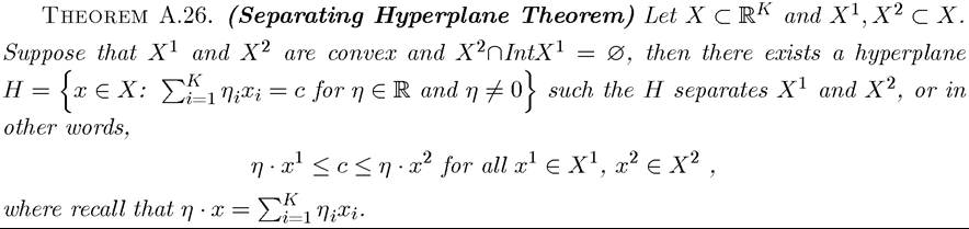
Note that the statement of this theorem disposes of the hypothesis that

which is not necessary when the two sets are subsets of Euclidean spaces. Moreover, the theorem does not add the qualification that the hyperplane H is “nonzero” (in the same way as Theorem A.25 did for linear functionals), since the definition of the hyperplane already incorporates this requirement.

A.10. Constrained Optimization

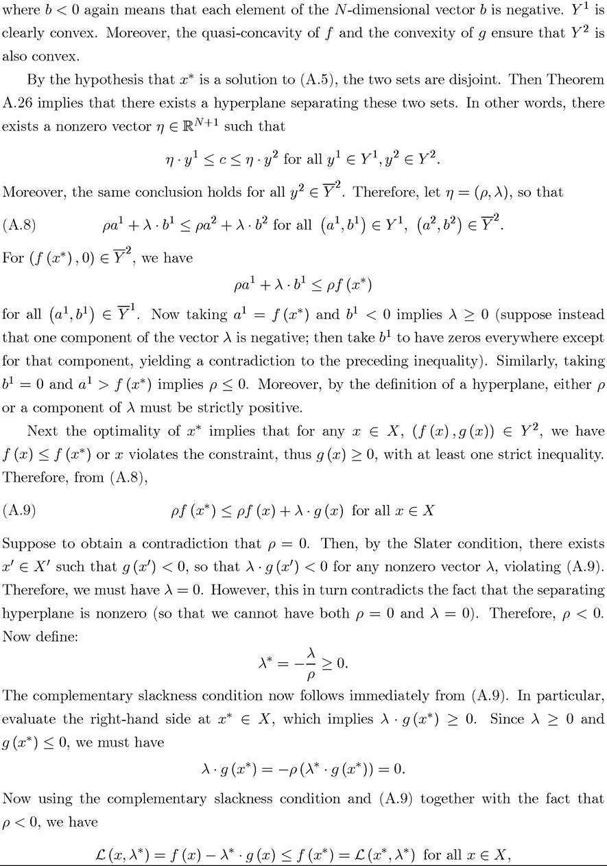
Many of the problems we encountered in this book are formulated as constrained optimiza­tion problems. Chapters 6, 7, and 16 dealt with dynamic (infinite-dimensional) constrained optimization problems. Complementary insights about these problems can be gained by us­ing the separation theorems of the previous section. Let me illustrate this here by focusing on finite-dimensional optimization problems. In particular, suppose that X ⊂ R^k and consider the maximization problem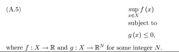

The constrained maximization problem (A.5) satisfies the Slater condition if there exists x' ∈ X such that g (x⁰) < 0 (meaning that each component of the mapping g takes a negative value). This is equivalent to the set G = {x:g (x) ≤ 0} having an interior point. We say that g is convex, if each component function of g is convex. This implies that the set G is also convex (but the converse is not necessarily true (see Exercise A.33).As is usual, we define the Lagrangian function as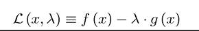

forThe vector λ is referred to as the Lagrange multiplier. Note also that λ ∙ g (x)

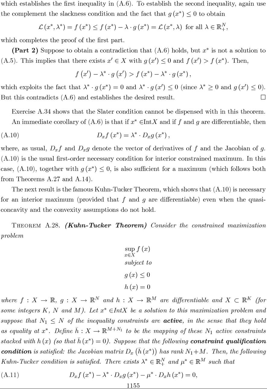
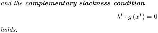
denotes the inner product of the two N dimensional vectors. A central theorem in constrained maximization is the following.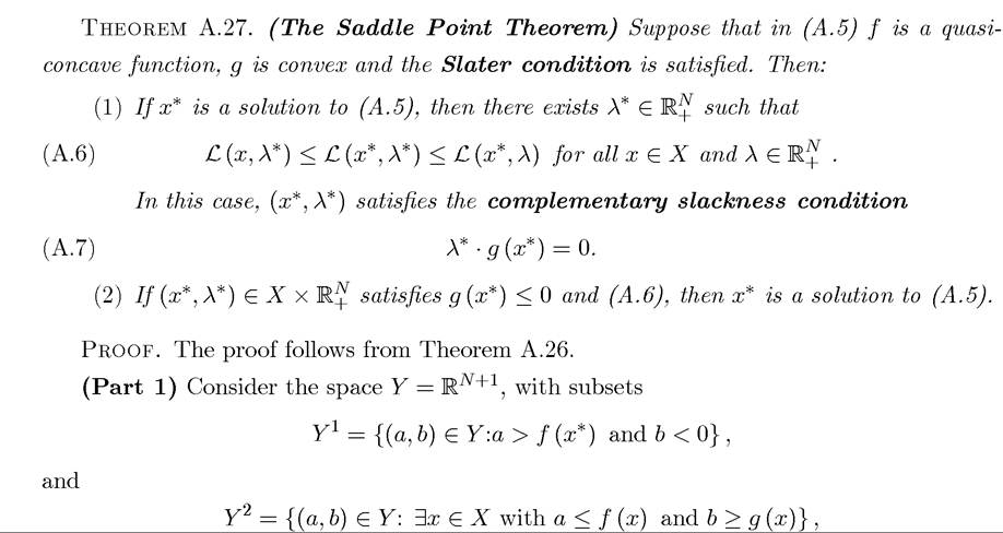

A.11. Exercises

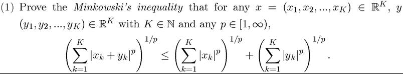
(2) Prove the generalization of this inequality for K = ∞.