Characterization of Equilibrium
8.2.1. Definition of Equilibrium. Let us now define an equilibrium in this dynamic economy. I provide two definitions, the first is somewhat more formal, while the second definition will be more useful in characterizing the equilibrium below.
Definition 8.1. A competitive equilibrium of the neoclassical growth model (Ramsey economy) consists of paths of consumption, capital stock, wage rates and rental rates of capital,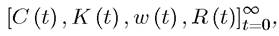 such that the representative household maximizes
its utility given initial asset holdings (capital stock) K (0) > 0 and the time path of prices [w (t),R (t)]∞o, and all markets clear.
Recall again that an equilibrium corresponds to the entire time path of real quantities and the associated prices. We may sometimes focus on the steady-state equilibrium, but equilibrium always refers to the entire path.
Since everything can be equivalently defined in terms of per capita variables, an alternative and more convenient definition of equilibrium is as follows:
Definition 8.2. A competitive equilibrium of the neoclassical growth model (Ramsey economy) consists of paths of per capita consumption, capital-labor ratio, wage rates and 322
8.2.2. Household Maximization. Let us start with the problem of the representative household. From the definition of equilibrium we know that this is to maximize (8.3) subject to (8.8) and (8.14). This is a special case of discounted infinite-horizon control problems discussed in Theorem 7.13 in the previous chapter. To derive the necessary conditions for an optimal consumption-saving plan for the household, let us set up the current-value Hamiltonian:

with state variable a, control variable c and current-value costate variable μ.
This problem is closely related to the problem of optimal growth already discussed in Section 7.7 in the previous chapter, but with two main differences: first, the rate of return on assets is time varying; second, the terminal value constraint is represented by the no-Ponzi condition (8.14), which is slightly different from the one in Section 7.7, which was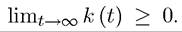 An
An argument similar to that in Section 7.7 makes sure that Theorem 7.13 can be applied to this problem (see Exercise 8.7).
Now applying Theorem 7.13, the necessary conditions for an interior solution are
and the transition equation (8.8). The transversality condition (the equivalent of (7.60) in the previous chapter) is

The transversality condition is written in terms of the current-value costate variable, which is more convenient given the rest of the necessary conditions. Note also that (8.16), (8.17) and (8.18) are necessary conditions for an interior solution. Are they also sufficient? Notice that, from (8.16), for any μ (t) > 0. This implies that H (t,a,c,μ) is a concave function of (a, c) (though not strictly so). Moreover, we will see that any (a (t),c (t)) that satisfies (8.14) must also satisfy so that the conditions of Theorem 7.14
are met. Therefore, conditions (8.16)-(8.18) are also sufficient and characterize a solution to the household maximization problem.
Let us now use these equations to derive a more explicit characterization. First, rearrange the second condition to obtain:
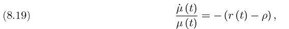
which states that the multiplier changes depending on whether the rate of return on assets is currently greater than or less than the discount rate of the household.
Next, the first necessary condition above implies that

To make more progress, let us differentiate the previous expression with respect to time and

Substituting this into (8.19) yields another form of the consumer Euler equation:

where

is the elasticity of the marginal utility u' (c(t)). This equation is closely related to the consumer Euler equation derived in the context of the discrete-time problem, eq. (6.36), as well as to the consumer Euler equation in continuous time with constant interest rates in Example 7.1 in the previous chapter. As with eq. (6.36), it states that consumption will grow over time when the discount rate is less than the rate of return on assets. It also specifies the speed
at which consumption will grow in response to a gap between this rate of return and the discount rate, which is related to the elasticity of marginal utility of consumption, εu (c (t)). The interpretation of εu (c (t)) and of this equation will be discussed further below.
Next, integrating eq. (8.19),
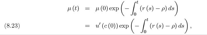
where the first line uses the form of the solutions to linear nonhomogeneous differential equations (see Section B.4 in Appendix Chapter B), and the second line uses (8.16) evaluated at time t = 0. Substituting (8.23) into the transversality condition yields
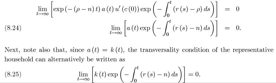
This equation emphasizes that the transversality condition requires the discounted market value of the capital stock in the very far future to be equal to 0.
This “market value” version of the transversality condition is both intuitive and often more convenient to work with.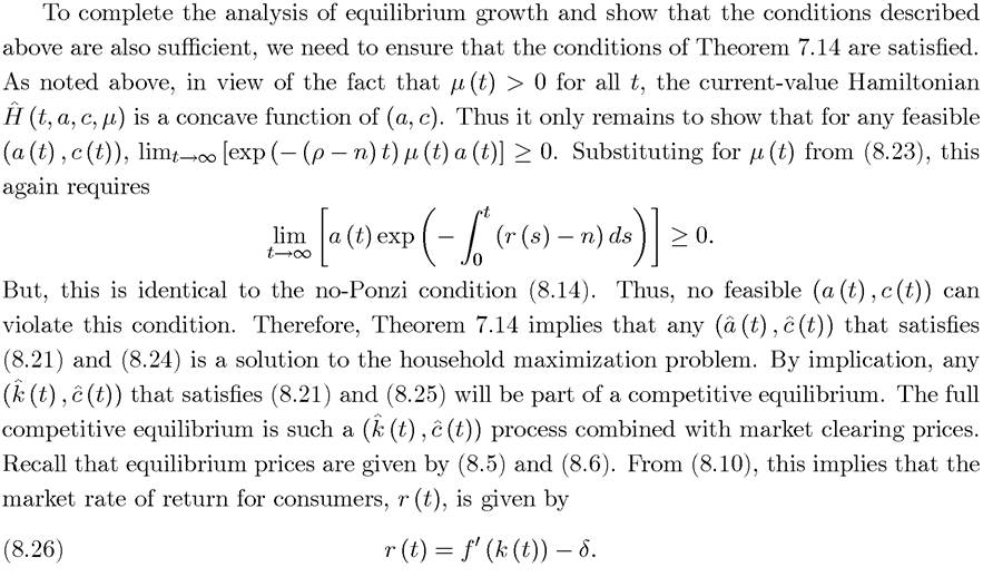
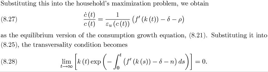
Conditions (8.27) and (8.28) are expressed only in terms of the path of the capital-labor ratio and fully characterize a competitive equilibrium. Moreover, we will see shortly that this competitive equilibrium is unique and that these conditions are identical to the Euler equation and the transversality condition in the optimal growth problem (see Exercise 8.11).
8.2.3. Consumption Behavior. Let us now return to the dynamics of the representative household’s consumption. First, recall that the Euler equation, (8.21), relates the “slope” of the consumption profile of the households to which was de fined as the
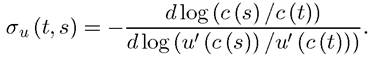
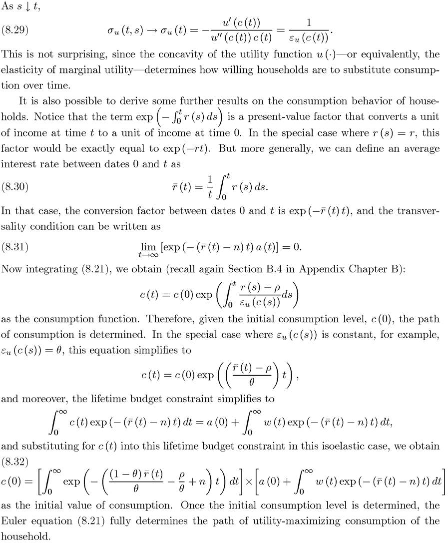
elasticity of the marginal utility function, u' (c). Notice, however, that is not only the elasticity of marginal utility, but even more importantly, it is the inverse of the intertemporal elasticity of substitution, which plays a crucial role in macro models. The intertemporal elasticity of substitution regulates the willingness of households to substitute consumption (or labor or any other attribute that yields utility) over time. The elasticity of marginal utility of consumption between the dates t and s > t is defined as
8.2.4. Using the Natural Debt Limit. Let us now return to the alternative approach of using the natural debt limit (8.12) instead of the no-Ponzi condition (8.14). In principle, ^ in (8.12) could be equal to minus infinity. However, exactly the same steps as in Exercise 8.2 show that this would violate the feasibility constraint that k (t) has to be nonnegative. In light of this, a well-defined equilibrium must involve ^ > -∞. We will see below that factor
8.3.