Preferences, Technology and Demographics

8.1.1. Basic Environment. Consider an infinite-horizon economy in continuous time and suppose that the economy admits a representative household with instantaneous utility function

The following standard assumption on this utility function will be maintained throughout the book unless stated otherwise.

Assumption 3. (Neoclassical Preferences) The utility function u (c) is defined on It is strictly increasing, concave, twice differentiable in the interior of its domain, with derivatives u' and u''.

More explicitly, the reader may wish to suppose that the economy consists of a set of identical households (with measure normalized to 1). Each household has an instantaneous utility function given by (8.1). Population within each household grows at the rate n, starting with L (0) = 1, so that total population in the economy is

All members of the household supply their labor inelastically.

Our baseline assumption is that the household is fully altruistic towards all of its future members, and always makes the allocations of consumption (among household members)

cooperatively. This implies that the objective function of each household at time t = 0, U (0), can be written as

where c (t) is consumption per capita at time t, ρ is the subjective discount rate, and the effective discount rate is ρ — n, since it is assumed that the household derives utility from the consumption per capita of its additional members in the future as well (see Exercise 8.1).

It is useful to be a little more explicit about where the objective function (8.3) is coming from. First, given the strict concavity of u (∙) and the assumption that within-household allocation decisions are cooperative, each household member will have an equal consumption (Exercise 8.1). This implies that each member will consume

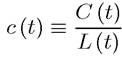
at date t, where C (t) is total consumption and L (t) is the size of the representative household (equal to total population, since the measure of households is normalized to 1). This implies that the household will receive a utility of u (c (t)) per household member at time t, or a total utility of L (t) u (c (t)) = exp (nt) u (c (t)). Since utility at time t is discounted back to time 0 with a discount rate of exp (—ρt), we obtain the expression in (8.3).

Let us also assume:

Assumption 4⁰. (Discounting)

This condition ensures that there is in fact discounting of future utility streams. Oth­erwise, (8.3) would have infinite value, and standard optimization techniques would not be useful in characterizing optimal plans. Assumption 4⁰ makes sure that in the model without growth, discounted utility is finite. When there is sustained growth, this condition will be strengthened to Assumption 4.

Let us start with an economy without any technological progress. Factor and product markets are competitive, and the production possibilities set of the economy is represented by the aggregate production function

Y (t) = F [K (t),L (t)],

which is a simplified version of the production function (2.1) used in the Solow growth model in Chapter 2. In particular, there is now no technology term (labor-augmenting technological change will be introduced below). As in the Solow model, Assumptions 1 and 2 are imposed throughout.

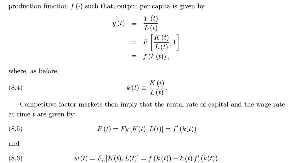
The demand side is somewhat more complicated, since each household will solve a continuous-time optimization problem in deciding how to use their assets and allocate con­sumption over time. To prepare for this, let us denote the asset holdings of the representative household at time t by A (t). Then, the law of motion for the total assets of the household is

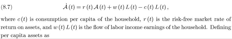
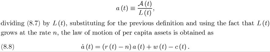
In practice, household assets can consist of (claims to) capital stock, K(t), which they rent to firms and government bonds, B (t). In models with uncertainty, households would have a portfolio choice between the capital stock of the corporate sector and riskless bonds (typically assumed to be supplied by the government). Bonds play an important role in models with incomplete markets, allowing households to smooth idiosyncratic shocks. Since these bonds are in zero net supply, in the aggregate B (t) = 0, and thus market clearing implies that assets per capita must be equal to the capital stock per capita. That is,

Because there is no uncertainty here, I ignore government bonds (until Chapter 17). Since household assets are the same as the capital stock and capital depreciates at the rate δ, the market rate of return on assets is

8.1.2. The Natural Debt Limit and the No-Ponzi Game Condition. Equation

(8.8) is a flow constraint. As already discussed in detail in Example 6.5 in Chapter 6, this flow constraint is not sufficient as a “proper budget constraint” on household behavior (unless we impose a lower bound on assets, such as a (t) ≥ 0 for all t, which is too strong; see Exercise 8.28).

(8.8), is not sufficient to capture the full set of constraints on household behavior.

There are two ways to proceed. The first is to impose the so-called “no-Ponzi condition,” which turns out to be the more convenient and flexible approach. The second involves imposing a natural debt limit (as in Example 6.5). Recall that the natural debt limit imposes that a (t) should never become so negative that the household cannot repay its debts even if it chooses zero consumption thereafter. Using (8.8) and assuming that the household does not consume from time t onwards, the natural debt limit in this case is found as

This is the direct analog of the discrete-time natural debt limit (6.41) in Chapter 6. In par­ticular, the right-hand side is the negative of the net present discounted value of labor income for the household. Exercise 8.3 asks you to work through a more detailed derivation of this condition. Any path of consumption and assets for the household that violates (8.11) is not feasible (unless we allow for bankruptcy). In view of this, the problem of the representative household can be expressed as the maximization of (8.3) subject to (8.8) and (8.11). In fact, one could simply impose the limiting version of this constraint,

This is because, if the natural debt limit is violated for some t' < ∞, then (8.12) cannot be satisfied either (see Exercise 8.4).

However, we will see below that the natural debt limit is not useful when we look at economies with sustained growth (because in that case ^ = -∞, see Exercise 8.8). For this reason, we must now undertake the investment for understanding the no-Ponzi game

condition. To start with, let us write the lifetime budget constraint of a household as

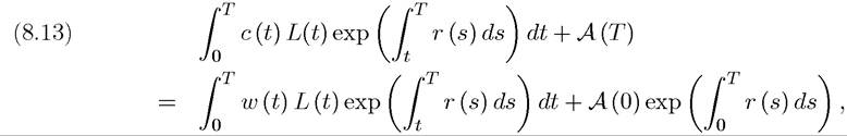
for some arbitrary T > 0. This constraint states that the household’s asset position at time T is given by his total income plus initial assets minus expenditures, all carried forward to date T units. Differentiating this expression with respect to T and dividing L(t) gives (8.8) (see Exercise 8.5).

Now imagine that (8.13) applies to a finite-horizon economy ending at date T. At this point, the household cannot have negative asset holdings, thus (8.13) must hold with A (T) ≥ 0. However, inspection of the flow budget constraint (8.8) makes it clear that this constraint does not guarantee A (T) ≥ 0. Therefore, in the finite horizon, we also need to impose A (T) ≥ 0 as an additional terminal value constraint.

In the infinite-horizon case, we need a similar constraint. The appropriate restriction is the no-Ponzi condition (or the no-Ponzi game condition). It takes the form

This condition is stated as an inequality, to ensure that the representative household does not asymptotically tend to a negative wealth. Intuitively, without (8.14), there is no proper lifetime budget constraint on the representative household (and by implication on any of the households in the economy) and they all increase their consumption by borrowing to such a level that feasibility is violated. This could clearly not be an equilibrium. At a more fundamental level, the relationship between the representative household and the financial markets must impose a proper lifetime budget constraint; otherwise financial markets would lose money.

The name “no-Ponzi condition” for (8.14) comes from the chain-letter or pyramid schemes, which are sometimes called Ponzi games, where an individual can continuously borrow from a competitive financial market (or more often, from unsuspecting souls that become part of the chain-letter scheme) and pay his or her previous debts using current bor­rowings. The consequence of this scheme would be that the asset holding of the individual would tend to -∞ as time goes by, violating feasibility at the economy level.

Let us momentarily return to the finite-horizon problem. In this case, financial markets would impose A (T) ≥ 0. But the household itself would never choose A (T) > 0, so the budget constraint could be simplified and written with A (T) = 0. In the same way, the no-Ponzi condition will imply

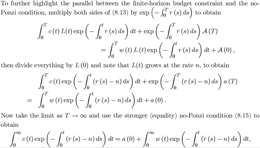
which requires the discounted sum of expenditures to be equal to initial income plus the discounted sum of labor income. Therefore this equation is a direct extension of (8.13) to infinite horizon. This derivation makes it clear that the no-Ponzi condition (8.14), or (8.15), essentially ensures that the household’s lifetime budget constraint holds in infinite horizon. In the analysis that follows, I will impose this constraint on household behavior.

8.2.