Comparative Dynamics
This section briefly undertakes some simple “comparative dynamics” exercises. Comparative dynamics are different from comparative statics in Propositions 2.3, 2.8 or 2.12 in that the focus is now on the entire path of adjustment of the economy following a shock or a change in parameters (rather than steady-state comparisons).
The basic Solow model is particularly well suited to such an analysis because of its simplicity. These exercises are also useful because the basic Solow model, and its neoclassical cousin, are often used for analysis of policy changes, medium-run shocks and business cycle dynamics, so an understanding of how the basic model responds to various shocks is useful in a range of applications.Recall that the law of motion of the effective capital-labor ratio in the continuous-time Solow model is given by (2.47) The right-hand side
of this equation is plotted in Figure 2.13. The intersection with the horizontal axis gives the unique steady-state (balanced growth) equilibrium, with effective capital-labor ratio k*. This figure is sufficient for the analysis of comparative dynamics. Consider, for example, a onetime, unanticipated, permanent increase in the saving rate from s to s'. This shifts the curve to the right as shown by the dashed line, with a new intersection with the horizontal axis at k**. The dashed arrows under the horizontal axis show how the effective capital-labor ratio adjusts gradually to the new balanced growth effective capital-labor ratio, k**. Immediately after the increase in the saving rate is realized, the capital stock and the effective capitallabor ratio remain unchanged (since they are state variables). After this point, k follows the dashed arrows and converges monotonically to
The comparative dynamics following a one-time, unanticipated, permanent decrease in δ or n are identical.
The same diagrammatic analysis can be used for studying the effect of an unanticipated, but transitory change in parameters. For example, imagine that s changes in an unanticipated manner at but this change will be reversed and the saving rate will return back to its original value at some known future date
 In this case, starting at t', the economy follows the dashed arrows until t'. After
 the original steady state of the differential equation applies and together with this the solid arrows above the horizontal axis become effective. Thus from
 onwards, the economy gradually returns back to its original balanced growth equilibrium, k*.
We will see that similar comparative dynamics can be carried out in the neoclassical growth model as well, but the response of the economy to some of these changes will be more complex.
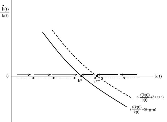
Figure 2.13. Dynamics following an increase in the savings rate from s to s'. The solid arrows show the dynamics for the initial steady state, while the dashed arrows show the dynamics for the new steady state.
2.9.