Solow Model with Technological Progress

2.7.1. Balanced Growth. The models analyzed so far did not feature technological progress. I now introduce changes in A (t) to capture improvements in the technological know-how of the economy.

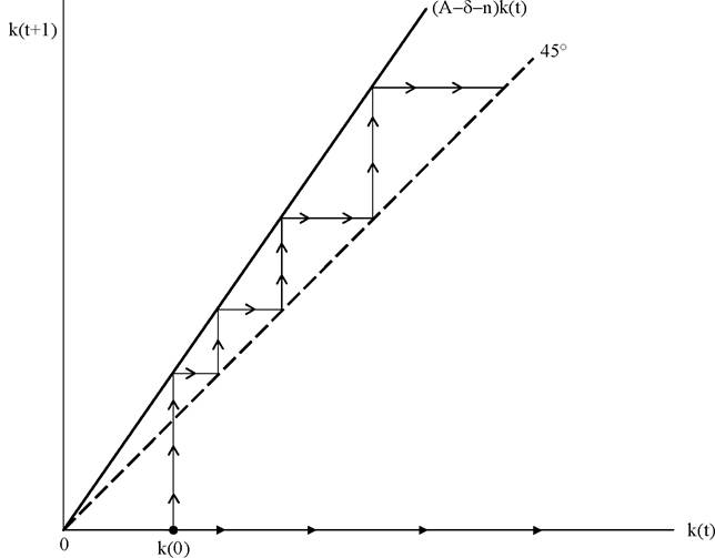
Figure 2.10. Sustained growth with the linear AK technology with sA — δ — n > 0.

that an attractive way of introducing economic growth in the framework developed so far is to allow technological progress in the form of changes in A (t). The question is how to do this. It turns out that the production functionis too general to achieve

our objective and may not lead to balanced growth. So our first task is to understand what types of restrictions need to be placed on F.

By balanced growth, we mean a path of the economy consistent with the Kaldor facts (Kaldor, 1963), that is, a path where, while output per capita increases, the capital-output ratio, the interest rate, and the distribution of income between capital and labor remain roughly constant. Figure 2.11, for example, shows the evolution of the shares of capital and labor in the US national income.

Despite fairly large fluctuations, there is no trend in these factors shares. Moreover, a range of evidence suggests that there is no apparent trend in interest rates over long time horizons and even in different societies (see, for example, Homer and Sylla, 1991). These facts and the relative constancy of capital-output ratios until the 1970s have made many economists prefer models with balanced growth to those without.

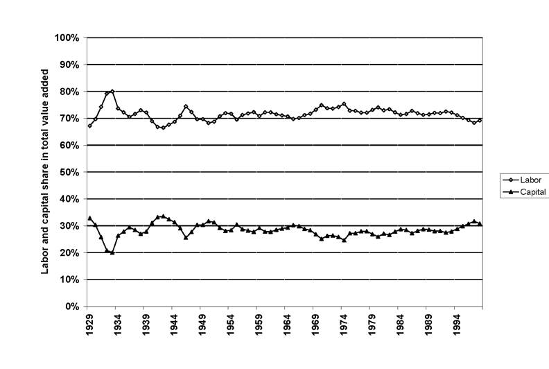
Figure 2.11. Capital and Labor Share in the U.S. GDP.

constant capital-output ratio are a good approximation to reality and a very useful starting point for our models.

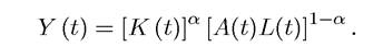
Also for future reference, note that the capital share in national income is about 1/3, while the labor share is about 2/3. This ignores the share of land: land is not a major factor of production in modern economies (though this is not true historically or for the less-developed economies of today). Exercise 2.12 illustrates how incorporating land into this framework changes the analysis. Note also that this pattern of the factor distribution of income, combined with economists’ desire to work with simple models, often makes them choose a Cobb-Douglas aggregate production function of the form AK¹Z³L²/³ as an approxi­mation to reality (especially since it ensures that factor shares are constant by construction). However, as Theorem 2.6 shows Cobb-Douglas technology is not necessary for constant factor shares or for balanced growth.

Why balanced growth? The most important reason to start with balanced growth is that it is much easier to handle than non-balanced growth, since the equations describing the law of motion of the economy can be represented by difference or differential equations with well- defined steady states. Put more succinctly, the main advantage of balanced growth is that it corresponds to a steady state of a transformed system (thus, balanced growth will imply k = O, except that now the definition of k will change). This will enable us to use the same tools used to analyze the steady states of stationary models to study economies with sustained 65

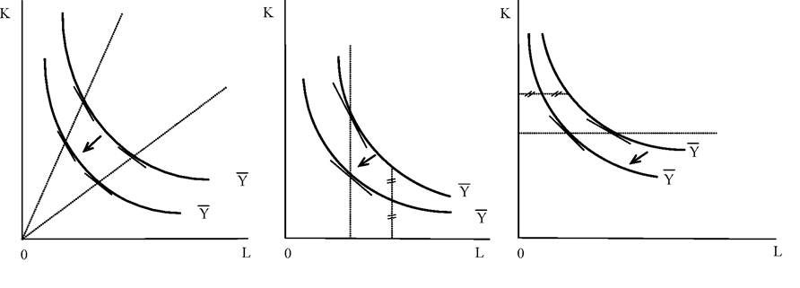
Figure 2.12.

growth. It is nonetheless important to bear in mind that in reality, growth has many non­balanced features. For example, the share of different sectors changes systematically over the growth process, with agriculture shrinking, manufacturing first increasing and then shrinking. Ultimately, we would like to have models that combine certain “balanced features” with these types of structural transformations. I will return to these issues in Part 7 of the book.

2.7.2. Types of Neutral Technological Progress. What are some convenient special 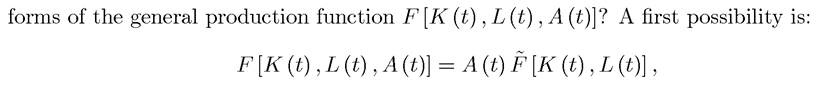for some constant returns to scale functionThis functional form implies that the tech­nology term A (t) is simply a multiplicative constant in front of another (quasi-) production function F and is referred to as Hicks-neutral after the famous British economist John Hicks. Intuitively, consider the isoquants of the functionspace,

which plot combinations of labor and capital for a given technology A (t) such that the level of production is constant. This is shown in Figure 2.12. Hicks-neutral technological progress, in the first panel, corresponds to a relabeling of the isoquants (without any change in their shape).

Another alternative is to have capital-augmenting or Solow-neutral technological progress, in the form

This is also referred to as capital-augmenting progress, because a higher A (t) is equivalent to the economy having more capital. This type of technological progress corresponds to the isoquants shifting inwards as if the capital axis is being “shrunk” (since a higher A now corresponds to a greater level of “effective capital”).

Finally, we can have labor-augmenting or Harrod-neutral technological progress, named after an early influential growth theorist Roy Harrod, who we encountered above in the context of the Harrod-Domar model previously:

This functional form implies that an increase in technology A (t) increases output as if the economy had more labor and thus corresponds to an inward shift of the isoquant as if the labor axis is being “shrunk”. The approximate form of the shifts in the isoquants are plotted in the third panel of Figure 2.12, again for a doubling of A (t).

Of course, in practice technological change can be a mixture of these, so we could have a vector valued index of technology A (t) = (A∏ (t),Ak (t),Al (t)) and a production function that looks like

which nests the constant elasticity of substitution production function introduced in Example 2.3 above. Nevertheless, even (2.41) is a restriction on the form of technological progress, since changes in technology, A (t), could modify the entire production function.

It turns out that, although all of these forms of technological progress look equally plau­sible ex ante, our desire to focus on balanced growth forces us to one of these types of neutral technological progress. In particular, balanced growth necessitates that all technological progress be labor-augmenting or Harrod-neutral. This is a very surprising result and it is also somewhat troubling, since there are no compelling reasons for why technological progress should take this form. I now state and prove the relevant theorem here and return to the discussion of why long-run technological change might be Harrod-neutral in Chapter 15.

2.7.3. The Steady-State Technological Progress Theorem.

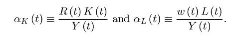
By Assumption 1 and Theorem 2.1, ακ (t) + (t) = 1.

The following theorem is a stronger version of a result first stated and proved by Uzawa and the proof builds on the argument developed in the recent paper by Schlicht (2006). It shows that asymptotic growth at constant rates (for output, capital and consumption) re­quires the aggregate production function to have a representation with Harrod-neutral tech­nological progress. Let us define an asymptotic path as a path of output, capital, consumption and labor as t → ∞.

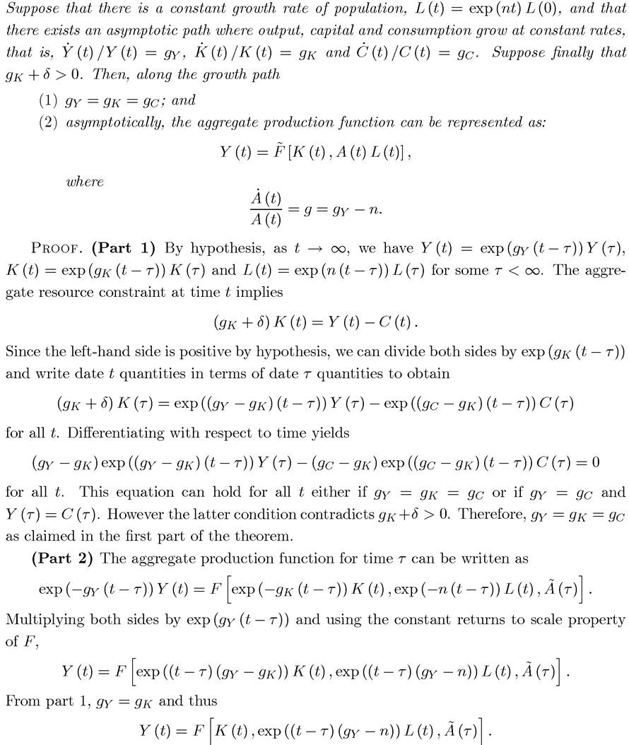
Theorem 2.6. (Uzawa^,s Theorem) Consider a growth model with a constant returns to scale aggregate production function

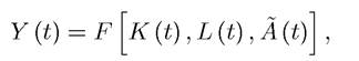
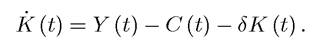
withrepresenting technology at time t and aggregate resource constraint

68

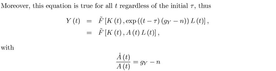
establishing the second part of the theorem. ?

A remarkable feature of this theorem is that it was stated and proved without any refer­ence to equilibrium behavior or market clearing. Also, contrary to Uzawa’s original theorem, it is not stated for a balanced growth path (meaning an equilibrium path with constant factor shares), but only for an asymptotic path with constant rates of output, capital and consump­tion growth.

Before providing a more economic intuition for this result, let us state an immediate implication of this theorem as a corollary, which will be useful both in the discussions below and for the intuition:

COROLLARY 2.3. Under the assumptions of Theorem 2.6, if an economy has an asymptotic path with constant growth of output, capital and consumption, then asymptotically technolog­ical progress can be represented as Harrod neutral (purely labor-augmenting).

The intuition for Theorem 2.6 and for the corollary is simple. We have assumed that the economy features capital accumulation in the sense that gκ + δ > 0. From the aggregate resource constraint, this is only possible if output and capital grow at the same rate. Either this growth rate is equal to the rate of population growth, n, in which case there is no technological change (the proposition applies with g = 0) or the economy exhibits growth of per capita income and capital-labor ratio. The latter case creates an asymmetry between capital and labor, in the sense that capital is accumulating faster than labor. Constancy of growth then requires technological change to make up for this asymmetry—that is, technology to take a labor-augmenting form.

This intuition does not provide a reason for why technology should take this labor­augmenting (Harrod-neutral) form, however. The theorem and its corollary simply state that if technology did not take this form, an asymptotic path with constant growth rates would not be possible. At some level, this is a distressing result, since it implies that bal­anced growth (in fact something weaker than balanced growth) is only possible under a very stringent assumption. Chapter 15 will show that when technology is endogenous the same intuition also implies that technology should be endogenously more labor-augmenting than capital-augmenting.

Notice also that this theorem does not state that technological change has to be labor­augmenting all the time. Instead, it requires that technological change ought to be labor­augmenting asymptotically (along the balanced growth path). This is exactly the pattern that certain classes of endogenous-technology models will generate.

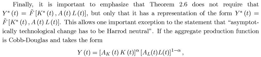
then both Ak (t) and Al (t) could grow asymptotically, while maintaining balanced growth. However, in this Cobb-Douglas example we can define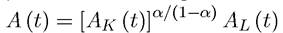and the

production function can be represented as

In other words, technological change can be represented as purely labor-augmenting, which is what Theorem 2.6 requires. Intuitively, the differences between labor-augmenting and capital-augmenting (and other forms) of technological progress matter when the elasticity of substitution between capital and labor is not equal to 1. In the Cobb-Douglas case, as we have seen above, this elasticity of substitution is equal to 1, thus different forms of technological progress are simple transforms of each other.

Another important corollary of Theorem 2.6 is obtained when we also assume that factor markets are competitive.

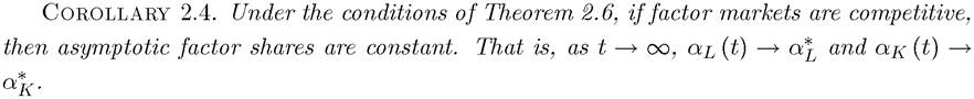
Proof. With competitive factor markets, we have that as t → ∞

where the second line uses the definition of the rental rate of capital in a competitive market, and the third line uses the fact that as t → ∞, gγ = gκ and gκ = g + n from Theorem 2.6 and that becauseexhibits constant returns to scale, its derivative with respect to K must be homogeneous of degree 0. ?

This corollary, together with Theorem 2.6, implies that any asymptotic path with constant growth rates for output, capital and consumption must be a balanced growth path and can

only be generated from an aggregate production function asymptotically featuring Harrod- neutral technological change.

In light of this corollary, we can provide further intuition for Theorem 2.6. Suppose the production function takes the special formThe corollary

implies that factor shares will be constant. Given constant returns to scale, this can only be the case when total capital inputsclass="lazyload" data-src="/files/uch_group77/uch_pgroup317/uch_uch7365/image/image162.jpg">and total labor inputs,grow

at the same rate; otherwise, the share of either capital or labor will be increasing over time. But if total labor and capital inputs grow at the same rate, then output Y (t) must also grow at this rate (because of constant returns to scale). The fact that the capital-output ratio is constant in steady state finally implies that K (t) must grow at the same rate as output and thus at the same rate as. Therefore, balanced growth is only possible if Ak (t) is

asymptotically constant.

2.7.4. The Solow Growth Model with Technological Progress: Continuous Time. I now present an analysis of the Solow growth model with technological progress in continuous time. The discrete-time case can be analyzed analogously and I omit the details to avoid repetition. Theorem 2.6 implies that asymptotically the production function must have a representation of the form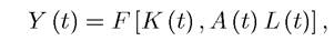

with purely labor-augmenting technological progress. For simplicity, I assume that it takes this form throughout. Moreover, suppose that there is technological progress at the rate g > 0, that is,

and population grows at the rate n as assumed in (2.32) above. Again using the constant saving rate we have

The simplest way of analyzing this economy is to express everything in terms of a nor­malized variable. Since “effective” or efficiency units of labor are given by A (t) L (t), and F exhibits constant returns to scale in its two arguments, I now define k (t) as the effective capital-labor ratio (capital divided by efficiency units of labor) so that

Differentiating this expression with respect to time,

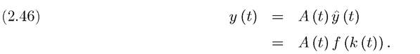
The quantity of output per unit of effective labor can be written as

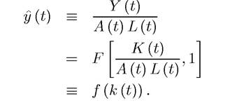
Income per capita is y (t) ? Y (t) /L (t), so that

It should be clear that ifis constant, income per capita, y (t), will grow over time, since A (t) is growing. This highlights that in this model, and more generally in models with technological progress, we should not look for “steady states” where income per capita is con­stant, but for balanced growth paths, where income per capita grows at a constant rate, while some transformed variables such asor k (t) in (2.45) remain constant. Since these trans­formed variables remain constant, balanced growth paths can be thought of as steady states of a transformed model. Motivated by this observation, in models with technological change throughout I will use the terms “steady state” and balanced growth path interchangeably.

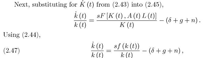
which is very similar to the law of motion of the capital-labor ratio in the model without technological progress, (2.33). The only difference is the presence of g, which reflects the fact that now k is no longer the capital-labor ratio but the effective capital-labor ratio and thus for k to remain constant in the balanced growth path, the capital-labor ratio needs to increase at the rate g.

An equilibrium in this model is defined similarly to before. A steady state or a balanced growth path is, in turn, defined as an equilibrium in which the effect of capital-labor ratio k (t) is constant. Consequently (proof omitted):

PROPOSITION 2.11. Consider the basic Solow growth model in continuous time with Harrod-neutral technological progress at the rate g and population growth at the rate n. Sup­pose that Assumptions 1 and 2 hold, and define the effective capital-labor ratio as in (2.44). Then, there exists a unique steady state (balanced growth path) equilibrium where the effective capital-labor ratio is equal to k* ∈ (0, ∞) given by

Per capita output and consumption grow at the rate g.

Equation (2.48), which determines the steady-state level of the effective capital-labor ratio, emphasizes that now total savings, sf (k), are used for replenishing the capital stock for three distinct reasons. The first is again the depreciation at the rate δ. The second is population growth at the rate n, which reduces capital per worker. The third is Harrod- neutral technological progress at the rate g, reducing effective capital-labor ratio at this rate when the capital-labor ratio is constant. Thus the replenishment of the effective capital-labor ratio requires investments to be equal to (δ + g + n) k, which is the intuitive explanation for eq. (2.48).

The comparative static results are also similar to before, with the additional comparative static with respect to the initial level of the labor-augmenting technology, A (0) (the level of technology at all points in time, A (t), is completely determined by A (0) given the assumption in (2.42)). We therefore have:

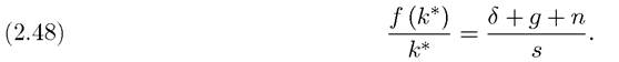
Proposition 2.12. Suppose Assumptions 1 and 2 hold and let A (0) be the initial level of technology. Denote the balanced growth path level of effective capital-labor ratio by k* (A (0),s,δ, n) and the level of output per capita by y* (A (0),s,δ,n,t) (the latter is a func­tion of time since it is growing over time). Then,

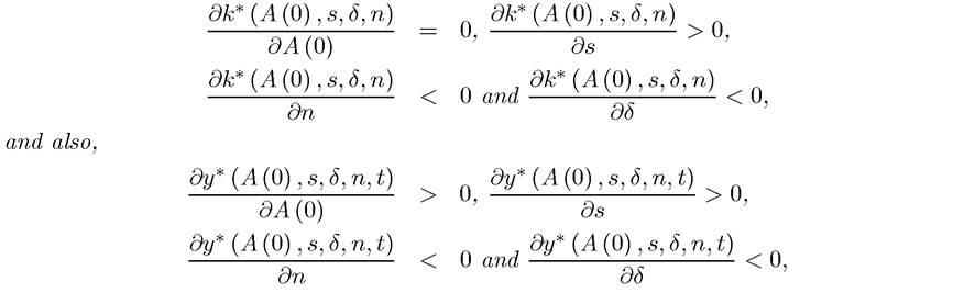
for each t.

Proof. See Exercise 2.21.

Finally, the transitional dynamics of the economy with technological progress are similar to the dynamics without technological change.

PROPOSITION 2.13. Suppose that Assumptions 1 and 2 hold, then the Solow growth model with Harrod-neutral technological progress and population growth in continuous time is asymp­totically stable, that is, starting from any k (0) > 0, the effective capital-labor ratio converges to a steady-state value k* (k (t) → k*).

Proof. See Exercise 2.22. ?

Therefore, the comparative statics and dynamics are very similar to the model without technological progress. The major difference is that now the model generates growth in output per capita, so it can be mapped to the data much better. However, the disadvantage is that growth is driven entirely exogenously. The growth rate of the economy is exactly 73

the same as the exogenous growth rate of the technology stock. The model specifies neither where this technology stock comes from nor how fast it grows.

2.8.