Consumption and Portfolio Choice

The problem of how consumers choose between consumption and saving under uncertainty, in conjunction with the allocation of their portfolio among different assets, was first analyzed in an intertemporal setting by Samuelson [1969] and Merton [1969].

Assume a household that at time 0, maximizes an intertemporal utility function of the form

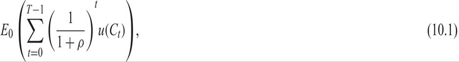
where E₀ denotes a mathematical expectation based on the set of available information available at time 0; ρ is the pure rate of time preference of the household; and u a one-period utility function, depending on the level of current consumption C_t.

The household is uncertain regarding its future income from employment and the future returns of its portfolio of assets. The evolution of the value of the household portfolio of assets is described by

where A_t is the value of the portfolio of assets of the household in the beginning of period t; Y_t is labor income, which is assumed to be a random variable whose value is known in period t. Gross savings of the household are defined by A_t + Y_t − C_t. The household allocates its gross savings between a safe asset with certain return r_t, and a risky asset with uncertain return x_t (x_t is assumed to be a random variable whose value is known in period t). The portfolio allocation decision of the household is determined by the percentage ω of its assets that is invested in the safe asset. The term in brackets in (10.2) thus denotes the average rate of return of the household’s portfolio.

The household chooses a consumption and portfolio allocation plan for period 0, knowing that it will be able to choose a new plan in the following period 1 on the basis on new information, a new plan in the following period 2, and so on, until the penultimate period T − 1. The easiest method of solving dynamic optimization problems under uncertainty is the method of stochastic dynamic programming.³

Dynamic programming converts multiperiod problems into a sequence of simpler two-period selection problems. The first step is the introduction of a value function V_t(A_t), which is defined as

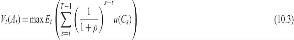
under the constraint (10.2).

The value function in period t is the discounted present value of the expected utility of the household, calculated under the assumption that the household follows the optimal program of consumption and portfolio allocation. This optimal value depends on the value of the portfolio of the household at the beginning of period t, which is the only state variable affecting the household. The value function depends of course on the conditional joint probability distribution of the random variables that describe the future labor income of the household and the uncertain rate of return of the risky asset, as well as the rate of return of the safe asset and the length of time between t and T −1. This dependence is indicated by the time index for the value function, and it shows that the value function may be changing over time.

From (10.3), the value function satisfies the following recursive equation, which is known as the Bellman equation:

The value function in period t is equal to the maximum utility of consumption in period t plus the discounted expected value function in period t + 1.

The first-order conditions for the maximization of the right-hand side of (10.4) under the constraint (10.2) are

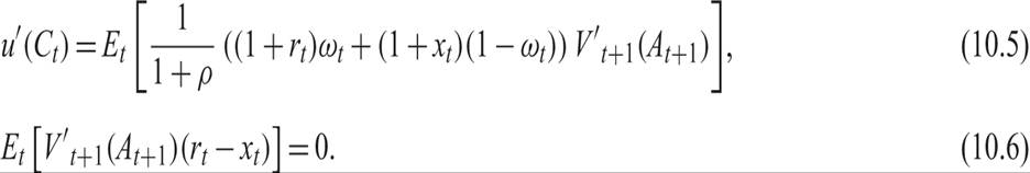
In (10.6), we have made use of the fact that the discounted gross savings of the household, which are equal to (A_t − Y_t − C_t)/(1 + ρ), are known in period t.

Applying the envelope theorem to (10.4) (i.e., the effects of a small change in the value of the portfolio of assets A_t on both sides of (10.4)), we get that

From (10.5) and (10.7), it follows that

The marginal value of the household portfolio of assets in the application of the optimal program is equal to the marginal utility of consumption. As a result, we can use (10.8) to substitute the marginal utility of future consumption for the marginal value of the future portfolio of assets in the first-order conditions (10.5) and (10.6):

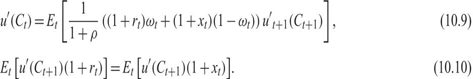
Substituting (10.10) in (10.9), the two conditions take the form

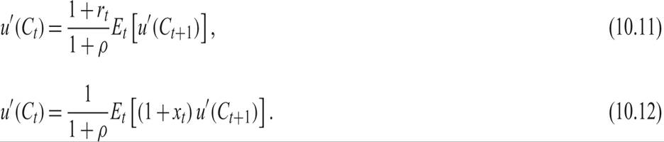
Conditions (10.11) and (10.12) have a simple interpretation, which is a generalization of the interpretation of the Euler equation for consumption in the Ramsey problem. Recall that the Euler equation for consumption in the Ramsey problem suggests that the marginal rate of substitution between the levels of consumption in the two periods must be equal to the marginal rate of transformation.

In the case of (10.11), assume that the household reduces its consumption by an infinitesimally small amount dC in period t, invests the amount in the safe asset, and consumes the return in the next period t + 1.

10.1.1 The Random Walk Model of Consumption

Equations (10.11) and (10.12) are just first-order conditions and do not describe the full solution of the problem. Nevertheless, they suggest strong restrictions for the dynamic behavior of consumption. Equation (10.11) implies that

where E_t(ε_t+1) = 0.

Equation (10.13) suggests that, given the marginal utility of consumption u′(C_t), no additional information is available in period t that could help predict u′(C_t+1), the future marginal utility of consumption.

Assuming that the utility function is quadratic in consumption and that the rate of return of the safe asset is equal to the pure rate of time preference, then (10.13) takes the form⁴

The model implies that consumption follows a random walk process. Given the level of consumption in period t, no other variable known in period t helps predict consumption in period t + 1. This prediction of the model was first highlighted by Hall [1978], who also investigated it empirically.

10.1.2 The Consumption Capital Asset Pricing Model

Conditions (10.11) and (10.12) can also be used to determine the rate of return of the risk-free asset and the expected rate of return (and hence the price) of the risky asset.

From (10.11), the rate of return of the risk-free asset will satisfy

From (10.12), it follows that

Cov denotes the covariance of two random variables.

From (10.16), the expected rate of return of the risky asset will satisfy

From (10.15) and (10.17), the expected return premium of the risky asset is given by

The expected return premium of the risky asset depends on the covariance of the rate of return of the risky asset with the marginal utility of consumption. Given that the marginal utility of consumption is negatively correlated with consumption, because of decreasing marginal utility, the expected return premium of the risky asset will depend positively on the covariance of the rate of return of this asset with consumption. Risky assets whose returns are positively correlated with consumption will tend to have a higher expected return relative to the risk-free asset.

This model of the determination of expected asset returns is known as the consumption capital asset pricing model (consumption CAPM).

10.2