Full Analysis of Consumption and Portfolio Choice

From the first-order conditions, one cannot fully describe the behavior of consumption and savings, apart from specific cases. One can come up with specific solutions for two special cases.

As demonstrated by Merton [1971], if labor income can be insured, we can deduce specific solutions for consumption for a broad class of utility functions, the hyperbolic absolute risk aversion (HARA) utility functions. This class includes isoelastic utility functions with constant relative risk aversion, the exponential utility function with constant absolute risk aversion, and quadratic utility functions.

One way to derive the specific solution is to use the Bellman principle of optimality, which says that for any value of the state variable (the portfolio of assets in this case) at a given time, the solution for the future must be optimal. Using this principle and the value function, the solution can be found through backward induction. For example, in period T − 2, for any value of the portfolio of assets A_T−2, the household faces a two-period problem. After solving this problem, take a step back, and solve the problem of the period T − 3, having already identified the value of the value function of T − 2. Then move on and solve the same problem inductively for the T − 4 period, and so on.

In the case of an infinite time horizon, take the limit of the solution to the problem of T periods as T tends to infinity. Alternatively, we can also solve the problem of infinite periods directly. For example, if the consumer has an infinite time horizon, the safe interest rate is fixed, and the uncertain return x_t is distributed according to an independent uniform probability distribution, then the value function is independent of time and only depends on the state variable A_t.

HARA utility functions allow us to infer analytical solutions, because the value function belongs to the same family as the utility function, and all that remains is to infer the parameters of the value function.

10.2.1 The Case of Logarithmic Preferences

Consider the simple case, in which

Using the result of Merton that the value function has the same functional form as the utility function for HARA utility functions, we assume that the value function takes the form

where a and b are constant parameters to be determined. This conjecture allows us to formulate the maximization problem in period t as

under the constraint⁵

Solving for consumption C and the share of the portfolio invested in the safe asset ω, we get

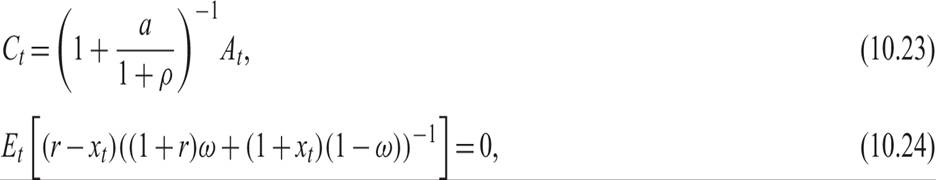
where (10.23) determines consumption as a linear function of the value of the total portfolio of assets of the household. Equation (10.24) determines indirectly the optimal proportion invested in the safe asset ω as a constant, due to the assumption that the return of the risky asset x is distributed according to a uniform independent probability distribution. The proportion ω is independent of the total value of the portfolio of assets.

To find a and b, substitute (10.22), (10.23), and (10.24) in the value function (10.21) and compare coefficients with (10.20).

In conclusion, assuming that labor income is insurable and the utility function is logarithmic, we get a consumption function analogous to the case of certainty. Consumption is a linear function of the total value of the portfolio of the household, and the marginal propensity to consume out of wealth depends only on the pure rate of time preference and not on the real interest rate or the rate of return of the risky asset. Changes in future nonlabor income (dividends and interest) affect consumption only through their impact on total wealth.

10.2.2 Quadratic Preferences and Certainty Equivalence

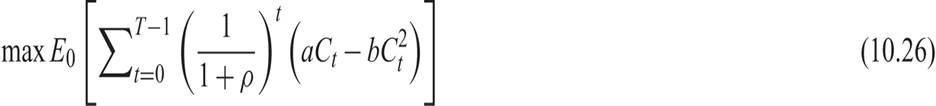
The second case we examine is the case of quadratic preferences. We initially assume that the portfolio consists only of the safe asset. The maximization problem of the household is

under the constraints

From the first-order conditions for a maximum, we have

In what follows, assume that r = ρ. In this case, (10.28) takes the form

which implies that

Because of the equality between the real interest rate and the pure rate of time preference, the optimal consumption path is such that there is perfect consumption smoothing.

The budget constraint (10.27) implies that

Because the household does not derive utility from its portfolio directly, but only from its consumption, its consumption in the last period will be such that A_T = 0. Using this transversality condition in (10.31), the intertemporal budget constraint of the household will be

According to (10.32), the present value of consumption of the household is equal to the value of its initial portfolio plus the present value of expected labor income. The household knows at time 0 that the budget constraint (10.32) should be satisfied but does not know future labor income. Accordingly, at time 0, the household aims to satisfy

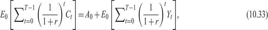
which suggests that the expected present value of consumption is equal to the value of the original portfolio of household plus the present value of expected labor income.

Substituting (10.30) in (10.33) and taking the limit as T tends to infinity results in

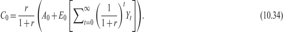
Consumption is constant and is a fixed percentage of the total wealth of the household, including the present value of expected labor income. In every period, the household consumes a constant fraction of its total wealth, depending on the real interest rate (or the pure rate of time preference), so that expected total wealth remains constant.

10.2.3 The Permanent-Income Hypothesis with Quadratic Preferences

From (10.30), the change in consumption from period to period is determined only by the revision of expectations regarding labor income:

For example, assume that labor income follows a stationary first-order autoregressive stochastic process (i.e., an AR(1) process) of the form

where a > 0 is a positive intercept, λ is the autoregressive parameter and satisfies 0 < λ < 1, and ε is a white noise process measuring the current innovation in labor income. Then one can show from (10.31) that the change in current consumption depends only on the current innovation in labor income ε.

By repeated substitutions we get

so that expected future innovations in current income depend only on the current innovation, with geometrically declining weights, determined by the autoregressive parameter λ.

Thus, assuming (10.36), when one calculates the geometric progression in (10.35) using the prediction formula above, the change in consumption is determined by

The coefficient of the transitory innovation in income ε is smaller than unity, because λ is less than unity. Equation (10.37) incorporates the predictions of the permanent-income hypothesis of Friedman [1957] and the life cycle hypothesis of Modigliani and Brumberg [1954] that consumption smooths out transitory changes in income.

If λ is equal to unity, then disturbances in labor income ε are of a permanent nature, and the coefficient of (10.37) is also equal to unity. Permanent changes in labor income lead to equal permanent changes in household consumption.

Empirical studies of the permanent income hypothesis suggest that aggregate consumption displays excess sensitivity to changes in current income, compared to the predictions of this hypothesis. This evidence suggests that one may have to go beyond the permanent-income hypothesis to adequately account for aggregate consumption.⁶

10.2.4 The Consumption CAPM with Quadratic Preferences

Assuming quadratic preferences, as we have in (10.26), the marginal utility of consumption is given by

The marginal utility of consumption is thus a negative linear function of consumption.

Substituting for the marginal utility of consumption in (10.18), we get

This confirms that under quadratic preferences, the expected return premium of a risky asset is proportional to the covariance of its return with consumption. This factor of proportionality is sometimes referred to as a consumption beta, from a regression of consumption growth on asset returns. Thus, a central prediction of the consumption CAPM is that the return premium of a risky asset is proportional to its consumption beta.⁷

However, empirical studies suggest an equity premium puzzle, that is, a much bigger difference between the average return of equities (the risky asset) and government bonds (the safe asset) than would be suggested by the consumption CAPM.⁸

10.2.5 The Efficient Markets Hypothesis

When the CAPM is combined with rational expectations on the part of investors, one gets a version of the efficient markets hypothesis (EMH). This hypothesis states that market participants make full use of available information in forming their expectations and therefore, the price of an asset fully reflects all available information.⁹

To demonstrate the logic of the EMH, assume a capital market in which investors choose between a common stock and a safe asset with a rate of return r. In equilibrium, optimality will ensure that the expected rate of return of the stock x will be equal to the rate of return of the safe asset plus a risk premium, as in (10.39). For simplicity, assume that both the rate of return of the safe asset r and the risk premium, denoted by σ, are constant:

where p is the price of the stock in the capital market, and d is the dividend. The expected rate of return of the stock E_t(x_t) is equal to the expected capital gain plus the dividend as a proportion of the stock price. In equilibrium in an efficient capital market, this cannot differ from the rate of return of the safe asset r plus the risk premium σ.

Equation (10.40) can be rearranged as

Under rational expectations, the fundamental solution of (10.41) gives us the stock price as the present value of current and expected future dividends, discounted by the sum of the rate of return of the safe asset and the risk premium σ:¹⁰

To find closed-form solutions, assume that dividends follow a stationary AR(1) process of the form

where is the steady state dividend, 0 < λ < 1 is the degree of persistence of deviations of current dividends from the steady state dividend, and ε_t+1 is a white noise process.

From (10.42) and (10.43), the fundamental solution is given by

From (10.44) and (10.43) it follows that

Thus the stock market price, based on fundamentals, is an AR(1) process itself, with mean equal to the present value of the steady state dividend /(r + σ).

From (10.45), it follows that

From (10.46), the current stock price fully reflects all available information about dividends. Hence, the only information relevant for predicting future stock prices is the current stock price itself. Only unanticipated changes in dividends (i.e., new information) can cause the future stock price to deviate from the currently expected future stock price.

Note that if dividends are nonstationary and follow a random walk (i.e., if λ = 1), then the stock price is a random walk itself, determined by

Equation (10.46) is modified accordingly and can be written as

If dividends follow a random walk process, stock prices follow a random walk process as well. In any case, the EMH suggests that no other variable apart from current stock prices helps predict future stock prices.¹¹

As with the consumption CAPM itself, the evidence on the EMH is generally mixed. The problem is that most empirical tests test a joint hypothesis: a model of asset pricing (such as the consumption CAPM) and the EMH. Thus it is hard to determine whether negative statistical tests imply rejection of the particular asset pricing model or the EMH. Both Fama and Shiller survey the empirical evidence in their Nobel lectures. Fama [2014] interprets the evidence as generally favorable to the EMH, but Shiller [2014] interprets the evidence as rejecting the EMH in favor of the alternative hypothesis of behavioral finance.¹²

10.3