Contracting Institutions and Technology Adoption

An important determinant of differences in technology and technology adoption are in­stitutional differences across societies. We have already noted how the parameter σj in the model of Section 18.2 can be interpreted as varying across countries because of differences in policies and institutions erecting barriers against technology adoption.

in providing a perspective in discussions. To make further progress, we need more micro­founded models of why there are barriers to technology adoptions and how these barriers affect technology choices. The reasons why certain groups may want to erect barriers against the introduction of new technologies will be discussed in detail in Part 8 below. In Part 7, we will discuss other factors affecting the efficiency of the organization of production, which can also be loosely related to “technology choices”. However, before turning to these models, it is useful to show how differences in the ability to write contracts between firms and their suppliers (or firms and their workers) may have first-order effect on technology adoption de­cisions. I will now briefly discuss a model of endogenous technology adoption, which again builds on the framework developed in Chapter 13. The purpose of this model is to illustrate how contractual difficulties can lead to important technological differences across countries and to emphasize the other side of the issue of technology adoption, i.e., how the conditions in the adopting country affect the use of these technologies by firms. The model I will present is a slight simplification of that by Acemoglu, Antras and Helpman (2007). The main focus is how differences in contracting institutions across countries will affect relationships between producers and suppliers and thus change the profitability of technology adoption.

18.5.1. Description of the Environment. For simplicity, consider a static world and focus on a single country. There exists a continuum of final goods q (z), with z ∈ [0,M], where M represents the number (measure) of final goods (I use M here, since N will denote

technology choice). All consumers have identical preferences,

where e is the total effort exerted by this individual, with ψ representing the cost of effort

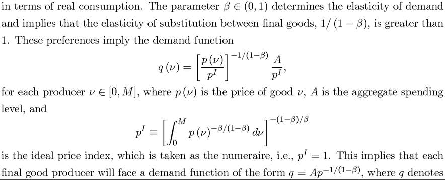
quantity and p denotes price, and I have dropped the conditioning on z, since I will focus on

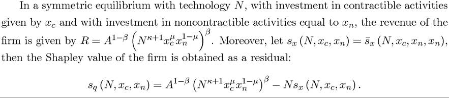
the decisions of a single firm. The resulting revenue function for the firm can therefore be written as

Production depends on the technology choice of the firm, which is denoted by N ∈ R₊. More advanced technologies involve a greater range of intermediate goods (inputs), supplied by different suppliers. The transactions between the producer and the suppliers will necessitate contracting relationships. For each j ∈ [0,N], let X (j) be the quantity of intermediate input j. The production function of the representative firm takes the standard CES form

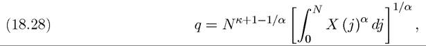
where we assume that 0 < a < 1, so that the elasticity of substitution between inputs, ε ? 1/ (1 — α), is always greater than one. In addition, we assume ê > 0. The standard specification of the CES (Dixit-Stiglitz) aggregator would not involve the term N^{κ+1- 1/a} (i.e., it would be implicitly setting κ = 1 /α — 1).

There is a large number of profit-maximizing suppliers that can produce the necessary intermediate goods. We assume that each supplier has the same outside option wo > 0. For now, let us take wo as given and also assume that each intermediate input needs to be produced by a different supplier with whom the firm needs to contract (see Exercise 18.31 on endogenizing this outside option). A supplier assigned to the production of an intermediate input needs to undertake relationship-specific investments in a unit measure of (symmetric) activities. The marginal cost of investment for each activity is ψ as specified in (18.26). The production function of intermediate inputs is Cobb-Douglas and symmetric in the activities:

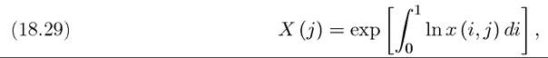
where x (i,j) is the level of investment in activity i performed by the supplier of input j. This formulation will allow a tractable parameterization of contractual incompleteness, whereby a subset of the investments necessary for production will be nonverifiable and thus noncontractible. Finally, we assume that adopting a technology N involves costs Γ (N), and impose the following two restrictions on Γ (N):

(i) For all N > 0, Γ (N) is twice continuously differentiable, with Γ⁰ (N) > 0 and Γ" (N) > 0.

These restrictions are standard. In particular, they introduce enough convexity to ensure interior solutions.

The relationship between the producer and its suppliers requires contracts to ensure that the suppliers deliver the required inputs. Let the payment to supplier j consist of two parts: an ex ante paymentbefore the investment levels x (i,j) take place, and a payment s (j) after the investments. Then, the payoff to supplier j, also taking account of her outside option, is

Similarly, the payoff to the firm is

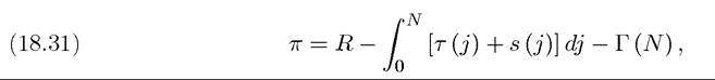
where R is revenue and the other two terms on the right-hand side represent costs. Substi­tuting (18.28) and (18.29) into (18.27), revenue can be expressed as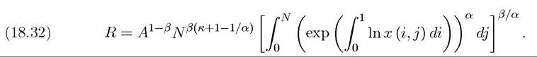

18.5.2. Equilibrium under Complete Contracts. As a benchmark, consider the “idealized” case of complete contracts, where the firm has full control over all investments and pays each supplier her outside option. Conceptually, complete contracts correspond to the case in which markets are complete, and intermediates of different qualities can be bought and sold in a quasi-competitive fashion. While this is a good approximation for many commodities, complete contracts (or the corresponding complete markets) may not always capture the essence of the interaction between firms and their suppliers, especially when contracting institutions are somewhat imperfect, so that using courts or other legal sanctions against firms that breach their contractual agreements might be costly.

To prepare for our treatment below of technology adoption under incomplete contracts, consider a game where the firm chooses a technology level N and makes a contract offer 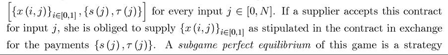combination for the firm and the suppliers such that suppliers maximize (18.30) and the firm maximizes (18.31).

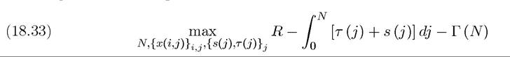
subject to (18.32) and the suppliers’ participation constraint,

Since the firm has no reason to provide rents to the suppliers, it chooses payments s (j) and τ (j) that satisfy (18.34) with equality. Moreover, with complete contracts, τ (j) and s (j) are perfect substitutes, so only the sum s (j) + τ (j) matters and is determined in equilibrium— this will not be the case when contracts are incomplete.

Moreover, since the firm’s objective function, (18.33), is (jointly) concave in the invest­ment levels x (i,j) and these investments are all equally costly, the firm chooses the same investment level x for all activities in all intermediate inputs. Now, substituting for (18.34) in (18.33), we obtain the following simpler unconstrained maximization problem for the firm:

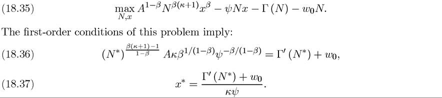
Equations (18.36) and (18.37) can be solved recursively. The restrictions on the function Γ above ensure that equation (18.36) has a unique solution for N*, which, together with

(18.37), yields a unique solution for x*.

When all the investment levels are identical and equal to x, output is q = N^κ+1x. Since a total of NX = Nx inputs are used in the production process, a natural measure of produc­tivity is output divided by total input use, P = N^κ. In the case of complete contracts this productivity level is

which is increasing in the level of technology. Summarizing this analysis, we have:

Proposition 18.9. Consider the above described model, take A as given and suppose that there are complete contracts.

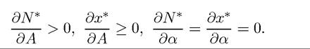
Proof. See Exercise 18.27. ?

In the case of complete contracts, the size of the market, which corresponds to A and from the viewpoint of the individual firm is exogenous, has a positive effect on investments by suppliers of intermediate inputs and productivity, because a greater market size makes 731

both suppliers’ and the producer’s investments more productive. The other noteworthy implication of this proposition is that under complete contracts, the level of technology and thus productivity do not depend on the elasticity of substitution between intermediate inputs, 1/ (1 - α).

18.5.3. Equilibrium under Incomplete Contracts. We now consider the same en­vironment under incomplete contracts. We model the imperfection of the contracting insti­tutions by assuming that there exists a μ ∈ [0,1] such that, for every intermediate input j, investments in activities 0 ≤ i ≤ μ are observable and verifiable and therefore contractible, while investments in activities μ < i ≤ 1 are not contractible. Consequently, a contract stipulates investment levels x (i,j) for the μ contractible activities, but does not specify the investment levels in the remaining 1 - μ noncontractible activities. Instead, suppliers choose their investments in noncontractible activities in anticipation of the ex post distribution of revenue, and may decide to withhold their services in these activities from the firm. In economies with weak contracting institutions, we will have a low μ, thus only a small set of tasks are contractible, whereas more developed contracting institutions will correspond to high levels of μ.

The ex post distribution of revenues in activities that are not ex ante contractible will be determined by multilateral bargaining between the firm and its suppliers. The exact bargaining protocol will determine investment incentives of suppliers and the profitability of investment for the firm. Below we will adopt the Shapley value as a natural solution concept for this multilateral bargaining game. First, consider the timing of events:

• The firm adopts a technology N and offers a contract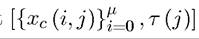for every

intermediate input j ∈ [0,N], where x_c (i, j) is an investment level in a contractible activity and τ (j) is an upfront payment to supplier j. The payment τ (j) can be positive or negative.

• Potential suppliers decide whether to apply for the contracts. Then the firm chooses N suppliers, one for each intermediate input j.

• All suppliers j ∈ [0,N] simultaneously choose investment levels x (i,j) for all i ∈ [0,1]. In the contractible activities i ∈ [0,μ] the suppliers will invest x (i,j) = ^χc ^(i,j).

• The suppliers and the firm bargain over the division of revenue, and at this stage, suppliers can withhold their services in noncontractible activities.

• Output is produced and sold, and the revenue R is distributed according to the bargaining agreement.

We will characterize a symmetric subgame perfect equilibrium (SSPE) of this game, where bargaining outcomes in all subgames are determined by Shapley values.

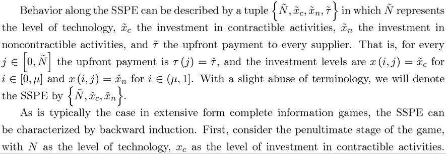
Equation (18.39) can be thought of as an “incentive compatibility constraint,” with the additional symmetry requirement. While this equation is written with ^t∈ to allow for the fact that there may be more than one maximizers of the expression on the right-hand side, the structure of the current model ensures that there will be a unique maximizer, thus “+’ can be replaced with the equal sign, “=”.

Now consider the stage in which the firm chooses N suppliers from a pool of applicants. If suppliers expect to receive less than their outside option, wo, this pool is empty. Therefore, for production to take place, the final-good producer has to offer a contract that satisfies the participation constraint of suppliers under incomplete contracts, i.e.,

In other words, given N and (x_c,τ), each supplier j ∈ [0,N] should expect her Shapley value plus the upfront payment to cover the cost of investment in contractible and noncontractible activities and the value of her outside option.

The maximization problem of the firm can then be written as:

subject to (18.39) and (18.40).

With no restrictions on τ, the participation constraint (18.40) will be satisfied with equal­ity; otherwise the firm could reduce τ without violating (18.40) and increase its profits. We can therefore solve τ from this constraint, substitute the solution into the firm’s objective function and obtain the simpler maximization problem:

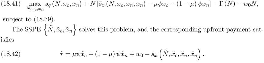
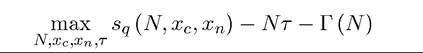
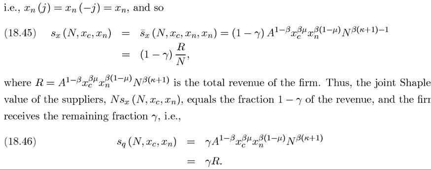
The key issue in the presence of incomplete contracts is that the payments from the firm to its suppliers will be determined ex post through bargaining rather than through contractual arrangements. As noted above, different bargaining protocols between suppliers and the producer will lead to somewhat different results. In the current context, the most natural choice appears to be the Shapley value, since it provides a plausible and tractable division rule for multilateral bargaining problems. The derivation of this formula is not essential for the results here, thus it is included for completeness at the end of this section. The next proposition provides the form of this bargaining solution.

Proposition 18.10. Suppose that supplier j invests x_n (j) in her noncontractible activ­ities, all the other suppliers invest x_n (—j) in their noncontractible activities, every supplier invests x_c in her contractible activities, and the level of technology is N. Then the Shapley

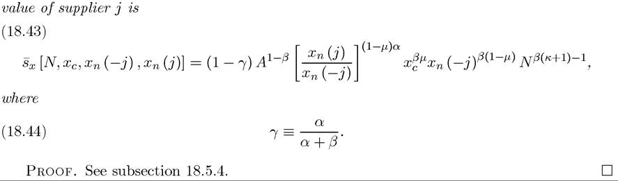
A number of features of (18.43) are worth noting. First, the derived parameter γ ? α/ (α + β) represents the bargaining power of the firm; it is increasing in α and decreasing in β. A higher elasticity of substitution between intermediate inputs, i.e., a higher α, raises the firm’s bargaining power, because it makes every supplier less essential in production and therefore raises the share of revenue appropriated by the firm. In contrast, a higher elasticity of demand for the final good, i.e., higher β, reduces the firm’s bargaining power, because, for any coalition, it reduces the marginal contribution of the firm to the coalition’s payoff as a fraction of revenue.

Second, in equilibrium, all suppliers invest equally in all the noncontractible activities,

^y

n

This is a relatively simple rule for the division of revenue between the firm and its suppliers.

Finally, when α is smaller,is more concave with respect to

x_n (j), because greater complementarity between the intermediate inputs implies that a given change in the relative employment of two inputs has a larger impact on their relative marginal products. The impact of α on the concavity of s_x (∙) will play an important role in the following results. The parameter β, on the other hand, affects the concavity of revenue in output (see (18.27)), but has no effect on the concavity of s_x, because with a continuum of suppliers, a single supplier has an infinitesimal effect on output.

To characterize a SSPE, we first derive the incentive compatibility constraint using (18.39) and (18.43):

Relative to the producer’s first-best choice characterized above, we see two differences. First, the term (1 - γ) implies that the supplier is not the full residual claimant of the return from her investment in noncontractible activities and thus underinvests in these activities. Second, as discussed above, multilateral bargaining distorts the perceived concavity of the private return relative to the social return. Using the first-order condition of this problem 735

and solving for the fixed point by substituting x_n (j) = x_n yields a unique x_n:

This equation implies that investments in noncontractible activities are increasing in α. Math­ematically, this follows from the fact that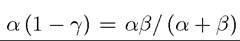is increasing in α. The

economics of this relationship is the outcome of two opposing forces. The share of the suppliers in revenue,, is decreasing in α, because greater substitution between the intermediate inputs reduces the suppliers’ ex post bargaining power. But a greater level of α also reduces the concavity ofin x_n, increasing the marginal reward from investing further in noncontractible activities. Because the latter effect dominates, x_n is increasing in α.

Another interesting feature is that contractible and noncontractible activities are com­plements, and in particular, X_n (N, x_c) is increasing in x_c. Finally, the effect of N on x_n is ambiguous, since investment in noncontractible activities declines with the level of technology when β (κ + 1) < 1 and increases with N when β (κ + 1) > 1. This is because an increase in N has two opposite effects on a supplier’s incentives to invest; a greater number of inputs increases the marginal product of investment due to the “love for variety” embodied in the technology, but at the same time, the bargaining share of a supplier,declines

with N. For large values of κ the former effect dominates, while for small values of κ the latter dominates.

Now, using (18.45), (18.46) and (18.47), the firm’s optimization problem (18.41) can be expressed as the maximization of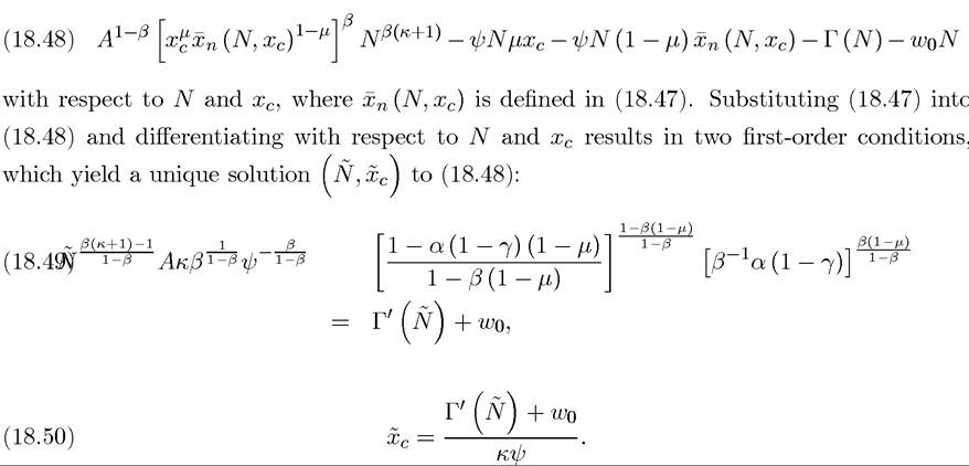

As in the complete contracts case, these two conditions determine the equilibrium recur­sively. First, (18.49) gives, and then given(18.50) yieldsMoreover, using (18.47), 736

(18.49), and (18.50) gives the level of investment in noncontractible activities as

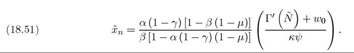
Comparing (18.37) to (18.50), we see that for a given N the implied level of investment in contractible activities under incomplete contracts, X_c, is identical to the investment level in contractible activities under complete contracts, x*. This highlights the fact that differences in investments in contractible activities between these economic environments only result from differences in technology adoption. In fact, comparing (18.36) with (18.49), we see that N and N* differ only because of the two bracketed terms on the left-hand side of (18.49). These represent the distortions created by bargaining between the firm and its suppliers. Intuitively, technology adoption is distorted because incomplete contracts reduce investments in noncontractible activities below the level of investment in contractible activities and this

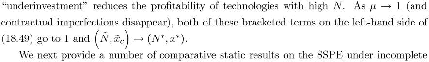
contracts and compare the incomplete-contracts equilibrium to the equilibrium under com­plete contracts. The comparative static results are facilitated by the block-recursive structure of the equilibrium; any change in A, μ or α that increases the left-hand side of (18.49) also increaseand the effect on x_c and x_n can then be obtained from (18.50) and (18.51). The main results are provided in the next proposition:

PROPOSITION 18.11. Consider the above described model with incomplete contracts and

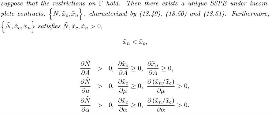
This proposition states that suppliers invest less in noncontractible activities than in

contractible activities. In particular, we have that

which follows from equations (18.50) and (18.51) and from the fact that α (1 — γ) = αβ/ (α + β) < β (recall (18.44)). This is intuitive: the producer firm is the full residual

claimant of the return to investments in contractible activities and it dictates these invest­

ments in the contract. In contrast, investments in noncontractible activities are decided by the suppliers, who are not the full residual claimants of the returns generated by these investments (recall (18.45)) and thus underinvest in these activities.

In addition, the level of technology and investments in both contractible and noncon- tractible activities are increasing in the size of the market, in the fraction of contractible activities (quality of contracting institutions), and in the elasticity of substitution between intermediate inputs. The impact of the size of the market is intuitive; a greater A makes production more profitable and thus increases investments and equilibrium technology. Bet­ter contracting institutions, on the other hand, imply that a greater fraction of activities receive the higher investment level X_c rather thanThis makes the choice of a more advanced technologies more profitable. A higher N, in turn, increases the profitability of fur­ther investments inBetter contracting institutions also close the (proportional)

gap between x_c andbecause with a higher fraction of contractible activities, the marginal

return to investment in noncontractible activities is also higher.

A higher α, i.e., lower complementarity between intermediate inputs, also increases tech­

nology choices and investments. The reason is related to the discussion in the previous subsection where it was shown that a higher α reduces the share of each supplier but also makes s_x (∙) less concave. Because the latter effect dominates, a lower degree of complemen­tarity increases supplier investments and makes the adoption of more advanced technologies more profitable.

One of the main implications of this analysis is that contractual frictions (here captured by the incomplete contracts equilibrium) lead to underinvestment in quality, discourage tech­nology adoption and reduce productivity. This is summarized in the next proposition. Note that productivity under incomplete contracts is, while productivity on the complete contracts, P*, is given in (18.38).

Proposition 18.12.be the unique SSPE with incomplete contracts and

let {N*,x*} be the unique equilibrium with complete contracts. Then

This proposition implies that since incomplete contracts lead to the choice of less ad­vanced (lower N) technologies, they also reduce productivity and investments in contractible and noncontractible activities. Acemoglu, Antras and Helpman (2007) also show that the technology and income differences resulting from relatively modest differences in contracting institutions can be quite large. Therefore, the link between contracting institutions and tech­nology adoption provides us with a theoretical mechanism that might generate significant technology differences across countries.

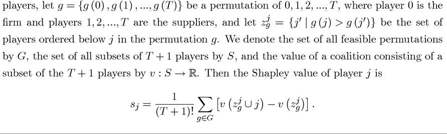
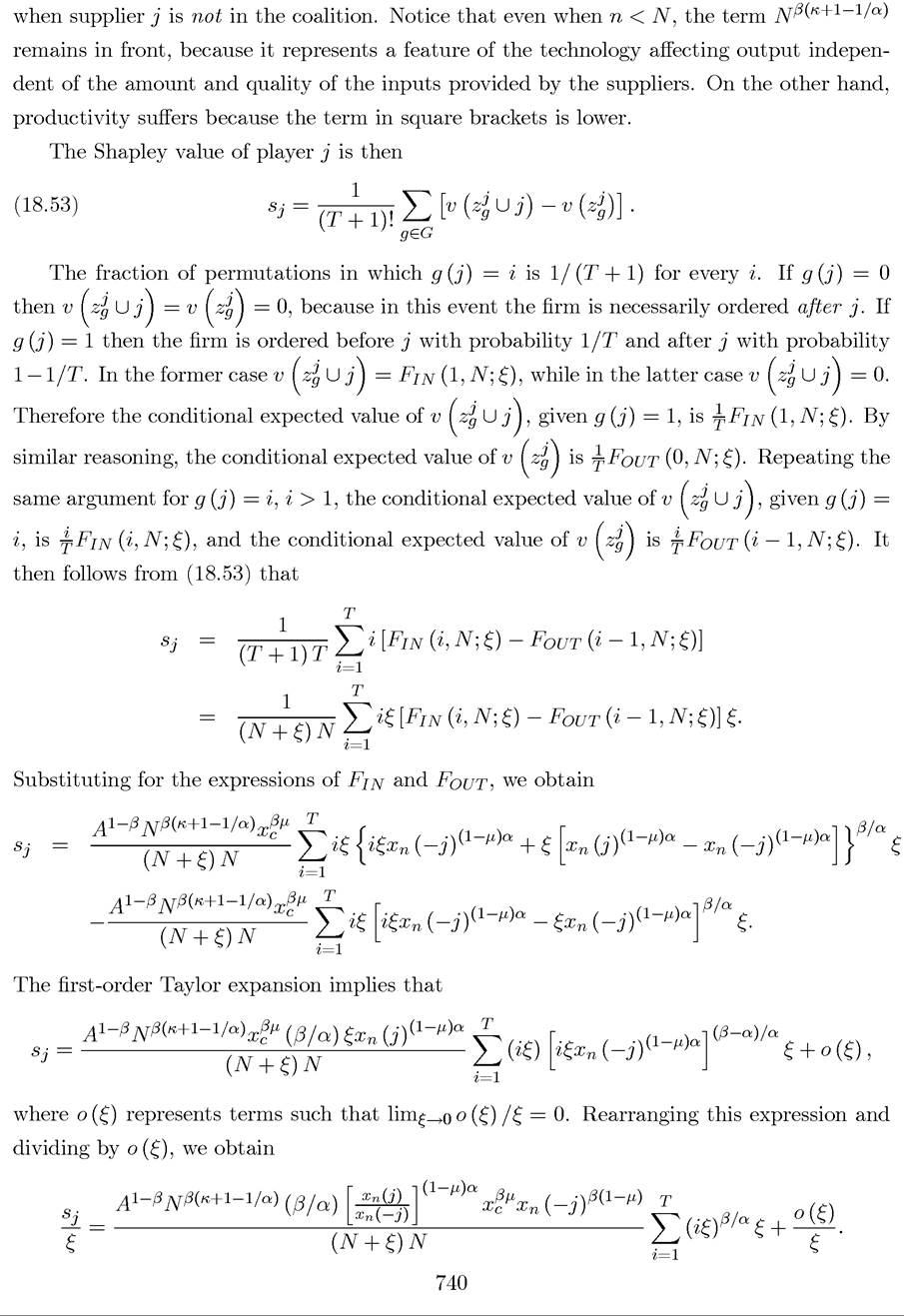
18.5.4. Appendix to Section 18.5: The Shapley Value and the Proof of Propo­sition 18.10 *. The concept of Shapley values, first proposed by Shapley (1953) has both intuitive and game theoretic appeal. In a bargaining game with a finite number of players, each player’s Shapley value is the average of her contributions to all coalitions that consist of players ordered below her in all feasible permutations. More explicitly, in a game with T +1

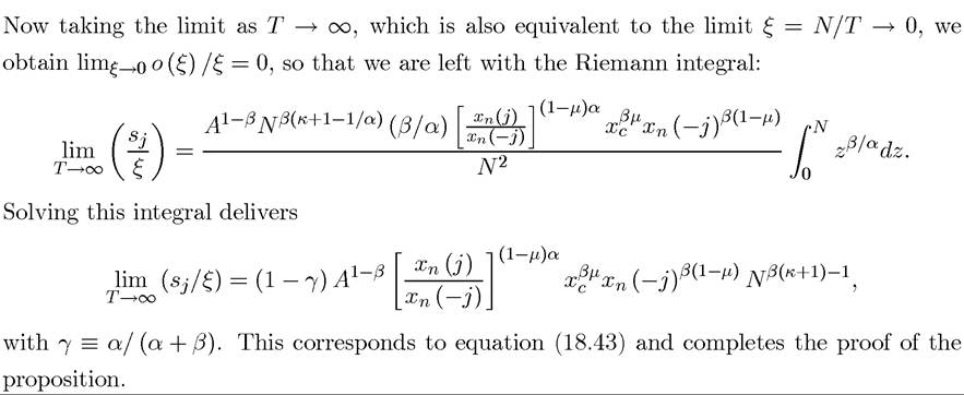
We now derive the asymptotic Shapley value proposed by Aumann and Shapley (1974), which involves considering the limit of this expression as the number of players goes to infinity. Let there be T suppliers each one controlling a range ξ = N/T of the continuum of intermediate inputs. Due to symmetry, all suppliers provide an amount x_c of contractible activities. As for the noncontractible activities, consider a situation in which a supplier j supplies an amount x_n (j) per noncontractible activity, while the T — 1 remaining suppliers supply the same amount x_n (—j) (note that we are again appealing to symmetry).

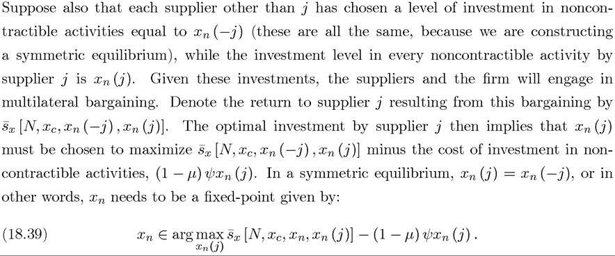
To compute the Shapley value for this particular supplier j, we need to determine the marginal contribution of this supplier to a given coalition of agents. A coalition of n suppliers and the firm yields a sales revenue of

when the supplier j is in the coalition, and a sales revenue

18.6.