Directed Technological Change with Knowledge Spillovers
I now consider the directed technological change model of the previous section with knowledge spillovers. This exercise has three purposes. First, it will show how the main results on the direction of technological change can be generalized to a model using the other common specification of the innovation possibilities frontier.
Second, this analysis will show that the strong bias result in Proposition 15.4 can hold under somewhat weaker conditions. Third, this formulation will be essential for the study of labor-augmenting technological change in Section 15.6.The lab-equipment specification of the innovation possibilities frontier is special in one respect: it does not feature for state dependence. State dependence refers to the phenomenon in which the path of past innovations affects the relative costs of different types of innovations. The lab-equipment specification implied that R&D spending always leads to the same increase in the number of L-augmenting and H -augmenting machines. I now introduce a specification 579
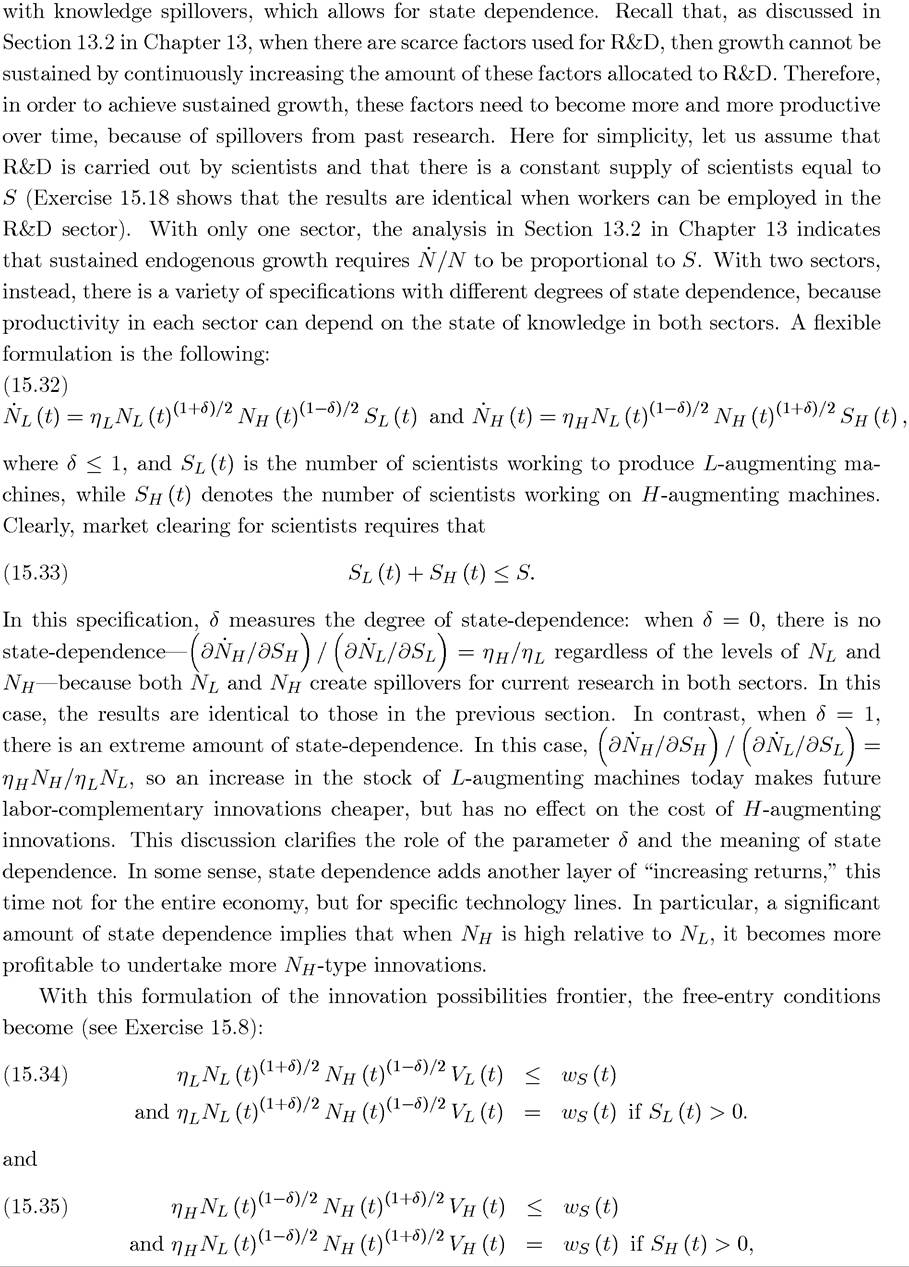
where ws (t) denotes the wage of a scientist at time t. When both of these free-entry conditions hold, BGP technology market clearing implies 
where δ captures the importance of state-dependence in the technology market clearing condition, and profits are not conditioned on time, since they refer to the BGP values, which are constant as in the previous section (recall (15.15)). When δ = 0, this condition is identical to (15.26) in the previous section. Therefore, as claimed above, all of the results concerning the direction of technological change would be identical to those from the lab-equipment specification.
This is no longer true when δ > 0. To characterize the results in this case, let us combine condition (15.36) with eq.’s (15.15) and (15.18). This yields the equilibrium relative technology as (see Exercise 15.9):
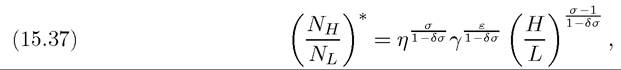
where recall that This expression shows that the relationship
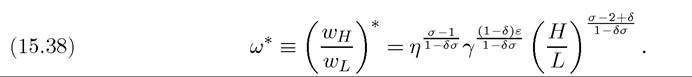
between the relative factor supplies and relative physical productivities now depends on δ. This is intuitive: as long as δ > 0, an increase in N∣∣ reduces the relative costs of H - augmenting innovations, so for technology market equilibrium to be restored, ∏l needs to fall relative to π∣∣. Substituting (15.37) into the expression for relative factor prices for given technologies, which is still given by (15.19), yields the following long-run (endogenous- technology) relationship between relative factor prices and relative factor supplies:
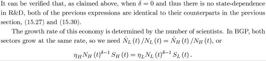
Combining this equation with (15.33) and (15.37), we obtain the following BGP condition for the allocation of researchers between the two different types of technologies,

In contrast to the model with the lab-equipments technology, transitional dynamics do not always take the economy to the BGP equilibrium, however. This is because of the additional increasing returns to scale mentioned above. With a high degree of state dependence, when Nh (0) is very high relative to Nl (0), it may no longer be profitable for firms to undertake further R&D directed at labor-augmenting (L-augmenting) technologies.
Whether this is so or not depends on a comparison of the degree of state dependence, 6, and the elasticity of substitution, σ. The latter matters because it regulates how prices change as there is an abundance of one type of technology relative to another, and thus determines the strength of the price effect on the direction of technological change. The next proposition analyzes the transitional dynamics in this case.
PROPOSITION 15.8. Consider the directed technological change model with knowledge spillovers and state dependence in the innovation possibilities frontier. Then, there is always weak equilibrium (relative) bias in the sense that an increase in H/L always induces relatively H-biased technological change.
Proof. See Exercise 15.13. ?
While the results regarding weak bias have not changed, inspection of (15.38) shows that it is now easier to obtain strong equilibrium (relative) bias.
PROPOSITION 15.9. Consider the directed technological change model with knowledge spil lovers and state dependence in the innovation possibilities frontier. Then, if  there is strong equilibrium (relative) bias in the sense that an increase in H/L raises the relative marginal product and the relative wage of the H factor compared to the L factor.
Intuitively, the additional increasing returns to scale coming from state dependence makes strong bias easier to obtain, because the induced technology effect is stronger. When a particular factor, say H, becomes more abundant, this encourages an increase in Nh relative to Nl (in the case where σ > 1). However, from state dependence, this makes further increases in Nh more profitable, thus has a larger effect on Nh/Nl. Since with σ > 1 greater values of Nh/Nl tend to increase the relative price of factor H compared to L, this tends to make the strong bias result easier to obtain.
Returning to the discussion of the implications of the strong bias results for the behavior of the skill premium in the US market, Proposition 15.9 implies that values of the elasticity of substitution between skilled and unskilled labor significantly less than 2 may be sufficient to generate strong equilibrium bias. How much lower than 2 the elasticity of substitution can be depends on the parameter δ. Unfortunately, this parameter is not easy to measure in practice, even though existing evidence suggests that there is some amount of state dependence in the R&D technologies. For example, this is confirmed by the empirical finding that most patents developed in a particular industry build upon and cite previous patents in the same industry.
15.5.