Discounted Infinite-Horizon Optimal Control
Part of the difficulty, especially regarding the absence of a transversality condition, comes from the fact that we did not impose enough structure on the functions f and g. As discussed above, our interest is with the growth models where the utility is discounted exponentially.
Consequently, economically interesting problems often take the following more specific form: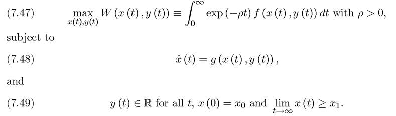
Notice that throughout we assume p > 0, so that there is indeed discounting.
The special feature of this problem is that the objective function, f, depends on time only through exponential discounting, while the constraint equation, g, is not a function of time directly. The Hamiltonian in this case would be:

where the second line defines
(7.50)
μ (t) ? exp (ρt) λ (t).
This equation makes it clear that the Hamiltonian depends on time explicitly only through the exp (-ρt) term.
In fact, in this case, rather than working with the standard Hamiltonian, we can work with the current-value Hamiltonian, defined as

which is “autonomous” in the sense that it does not directly depend on time.
The following result establishes the necessity of a stronger transversality condition under some additional assumptions, which are typically met in economic applications. In preparation for this result, let us refer to the functions f (x,y) and g (x,y) as weakly monotone, if each one is monotone in each of its arguments (for example, nondecreasing in x and nonincreasing in y). Furthermore, let us simplify the statement of this theorem by assuming that the optimal control y (t) is everywhere a continuous function of time (though this is not necessary for any of the results).
Theorem 7.14. (Maximum Principle for Discounted Infinite-Horizon Problems) Suppose that problem of maximizing (7.47) subject to (7.48) and (7.49), with f and g continuously differentiable, has a solution y (t) with corresponding path of state variable X (t). Suppose moreover that exists (where V (t,x (t)) is defined in (7.33)). Let
H(x,y,μ) be the current-value Hamiltonian given by (7.51). Then the optimal control y(t) and the corresponding path of the state variable X (t) satisfy the following necessary conditions:
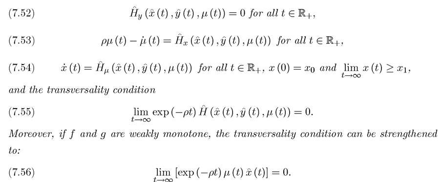
Proof. The derivation of the necessary conditions (7.52)-(7.54) and the transversality condition (7.55) follows by using the definition of the current-value Hamiltonian and from Theorem 7.13. They are left for as an exercise (see Exercise 7.13).
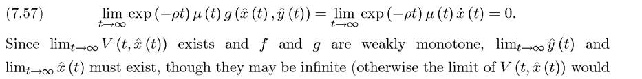
We therefore only give the proof for the stronger transversality condition (7.56). The weaker transversality condition (7.55) can be written as

The first term must be equal to zero, since otherwise
the pair cannot be reaching the optimal solution. Therefore
286
fail to exist). The latter fact also implies that limt→∞ x (t) exists (though it may also be infinite). Moreover, limt→∞ x (t) is nonnegative, since otherwise the condition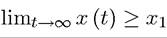
would be violated. From (7.53), (7.55) implies that as t → ∞,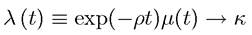 for
for
some
Suppose first that limt→∞ x (t) = 0.
Then . This
 also implies that and therefore
limit to constant values. Then from (7.52), we have that as t → ∞, μ (t) → μ* ∈ R (i.e., a finite value). This implies that κ = 0 and

and moreover since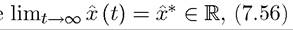 also follows.
Suppose now that :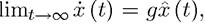 where g ∈ R+, so that x(t) grows at an expo
nential rate. Then substituting this into (7.57) we obtain (7.56).
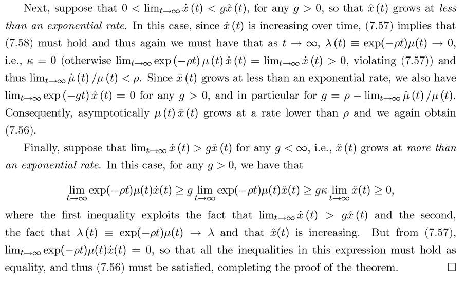
The proof of Theorem 7.14 also clarifies the importance of discounting. Without discounting the key equation, (7.57), is not necessarily true, and the rest of the proof does not go through.
Theorem 7.14 is the most important result of this chapter and will be used in almost all continuous time optimizations problems in this book. Throughout, when we refer to a discounted infinite-horizon optimal control problem, we mean a problem that satisfies all the assumptions in Theorem 7.14, including the weak monotonicity assumptions on f and g. Consequently, for our canonical infinite-horizon optimal control problems the stronger 287
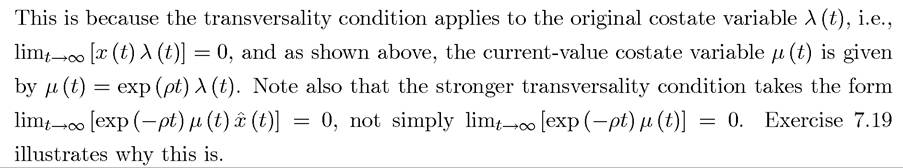
transversality condition (7.56) will be necessary. Notice that compared to the transversality condition in the finite-horizon case (e.g., Theorem 7.1), there is the additional term exp (—ρt).
The sufficiency theorems can also be strengthened now by incorporating the transversality condition (7.56) and expressing the conditions in terms of the current-value Hamiltonian:
Theorem 7.15.
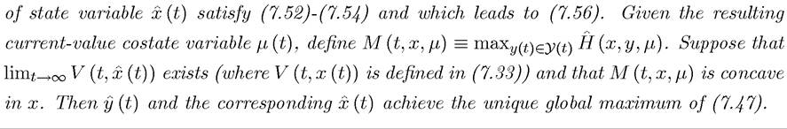
(Mangasarian Sufficient Conditions for Discounted InfiniteHorizon Problems) Consider the problem of maximizing (7.47) subject to (7.48) and (7.49), with f and g continuously differentiable and weakly monotone. Define H(x,y,μ) as the current-value Hamiltonian as in (7.51), and suppose that a solution y(t) and the corresponding path of state variable X(t) satisfy (7.52)-(7.54) and (7.56). Suppose also that exists and that for the resulting current-value costate variable μ (t),
 H (x,y,μ) is jointly concave in (x,y) for all , then y(t) and the corresponding X(t^) achieve the unique global maximum of (7.47).
Theorem 7.16. (Arrow Sufficient Conditions for Discounted Infinite-Horizon Problems) Consider the problem of maximizing (7.47) subject to (7.48) and (7.49), with f and g continuously differentiable and weakly monotone. Define H (x,y,μ) as the currentvalue Hamiltonian as in (7.51), and suppose that a solution y (t) and the corresponding path
The proofs of these two theorems are again omitted and left as exercises (see Exercise 7.12).
We next provide a simple example of discounted infinite-horizon optimal control.
EXAMPLE 7.3. One of the most common examples of this type of dynamic optimization problem is that of the optimal time path of consuming a non-renewable resource. In particular, imagine the problem of an infinitely-lived individual that has access to a non-renewable or exhaustible resource of size 1. The instantaneous utility of consuming a flow of resources y is u (y), where is a strictly increasing, continuously differentiable and strictly
concave function.
The individual discounts the future exponentially with discount rate p > 0, 288so that his objective function at time t = 0 is to maximize
The constraint is that the remaining size of the resource at time t, x (t) evolves according to
x (t) = —Ó (t),
which captures the fact that the resource is not renewable and becomes depleted as more of it is consumed. Naturally, we also need that x (t) ≥ 0.
The current-value Hamiltonian takes the form

Theorem 7.14 implies the following necessary condition for an interior continuously differentiable solution to this problem. There should exist a continuously differentiable
function μ (t) such that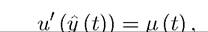 and
and
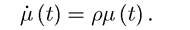
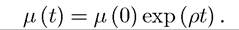
The second condition follows since neither the constraint nor the objective function depend on x (t). This is the famous Hotelling rule for the exploitation of exhaustible resources. It charts a path for the shadow value of the exhaustible resource. In particular, integrating both sides of this equation and using the boundary condition, we obtain that
Now combining this with the first-order condition for y (t), we obtain
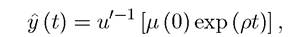
where is the inverse function of u', which exists and is strictly decreasing by virtue of the fact that u is strictly concave. This equation immediately implies that the amount of the resource consumed is monotonically decreasing over time.
Combining the previous equation with the resource constraint gives 
Integrating this equation and using the boundary condition that x (0) = 1, we obtain
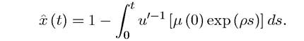
Since along any optimal path we must have limt→∞ x (t) = 0, we have that
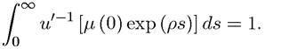
Therefore, the initial value of the costate variable μ (0) must be chosen so as to satisfy this equation.
Notice also that in this problem both the objective function, u (y (t)), and the constraint function, —y (t), are weakly monotone in the state and the control variables, so the stronger form of the transversality condition, (7.56), holds. You are asked to verify that this condition is satisfied in Exercise 7.22.
7.6.