Infinite-Horizon Optimal Control
The results presented so far are most useful in developing an intuition for how dynamic optimization in continuous time works. While a number of problems in economics require finite- horizon optimal control, most economic problems—including almost all growth models—are more naturally formulated as infinite-horizon problems.
This is obvious in the context of economic growth, but is also the case in repeated games, political economy or industrial organization, where even if individuals may have finite expected lifes, the end date of the game or of their lives may be uncertain. For this reason, the canonical model of optimization and economic problems is the infinite-horizon one.7.3.1. The Basic Problem: Necessary and Sufficient Conditions. Let us focus on infinite-horizon control with a single control and a single state variable. Using the same notation as above, the problem is
(7.28)
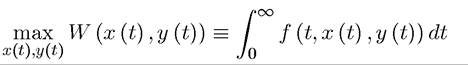
subject to
(7.29)
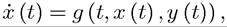
and
(7.30)

The main difference is that now time runs to infinity. Note also that this problem allows for an implicit choice over the endpoint xχ, since there is no terminal date. The last part of (7.30) imposes a lower bound on this endpoint. In addition, we have further simplified the problem by removing the feasibility requirement that the control y (t) should always belong to the set Y, instead simply requiring this function to be real-valued. Notice also that we have not assumed that the state variable x (t) lies in a compact set, thus the results developed here can be easily applied to models with exogenous or endogenous growth.
For this problem, we call a pair (x (t),y (t)) admissible if y (t) is a piecewise continuous function of time, meaning that it has at most a finite number of discontinuities.4 Since x (t) is given by a continuous differential equation, the piecewise continuity of y (t) ensures that x (t) is piecewise smooth. Allowing for piecewise continuous controls is a significant generalization of the above approach.
There are a number of technical difficulties when dealing with the infinite-horizon case, which are similar to those in the discrete time analysis. Primary among those is the fact that the value of the functional in (7.28) may not be finite. We will deal with some of these issues below.
The main theorem for the infinite-horizon optimal control problem is the following more general version of the Maximum Principle. Before stating this theorem, let us recall that the Hamiltonian is defined by (7.12), with the only difference that the horizon is now infinite. In addition, let us define the value function, which is the analog of the value function in discrete time dynamic programming introduced in the previous chapter:
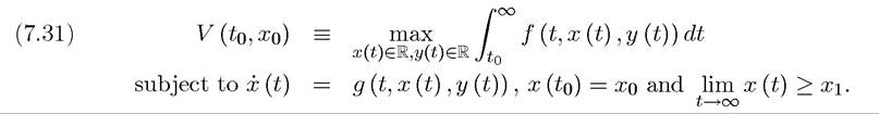
In words, V (to,xo) gives the optimal value of the dynamic maximization problem starting at time to with state variable xo. Clearly, we have that

Note that as in the previous chapter, there are issues related to whether the “max” is reached.
When it is not reached, we should be using “sup” instead. However, recall that we have
assumed that all admissible pairs give finite value, so that V (to,xo) < ∞, and our focus throughout will be on admissible pairs that are optimal solutions to (7.28) subject
to (7.29) and (7.30), and thus reach the value V (to,xo).
Our first result is a weaker version of the Principle of Optimality, which we encountered in the context of discrete time dynamic programming in the previous chapter:
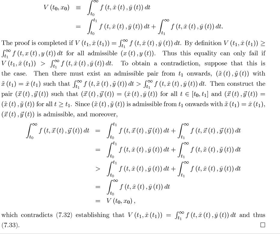
Lemma 7.1. (Principle of Optimality) Suppose that the pair (x (t),y (t)) is an optimal solution to (7.28) subject to (7.29) and (7.30), i.e., it reaches the maximum value V (to,xo). Then,
(7.33)
Proof. We have
Two features in this version of the Principle of Optimality are noteworthy. First, in contrast to the similar equation in the previous chapter, it may appear that there is no 275
discounting in (7.33). This is not the case, since the discounting is embedded in the instantaneous payoff function f, and is thus implicit in V (tι,x (tι)). Second, this lemma may appear to contradict our discussion of “time consistency” in the previous chapter, since the lemma is stated without additional assumptions that ensure time consistency. The important point here is that in the time consistency discussion, the decision-maker considered updating his or her plan, with the payoff function being potentially different after date tι (at least because bygones were bygones). In contrast, here the payoff function remains constant. The issue of time consistency is discussed further in Exercise 7.21. We now state one of the main results of this chapter.
Theorem 7.9. (Infinite-Horizon Maximum Principle) Suppose that problem of maximizing (7.28) subject to (7.29) and (7.30), with f and g continuously differentiable, has a piecewise continuous solution y (t) with corresponding path of state variable x(t). Let H (t,x,y,λ) be given by (7.12). Then the optimal control y (t) and the corresponding path of the state variable x (t) are such that the Hamiltonian H (t,x,y,λ) satisfies the Maximum Principle, that

for all t ∈ R.
Moreover, whenever y (t) is continuous, the following necessary conditions are satisfied: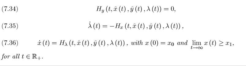
The proof of this theorem is relatively long and will be provided later in this section.[19] Notice that whenever an optimal solution of the specified form exists, it satisfies the Maximum Principle. Thus in some ways Theorem 7.9 can be viewed as stronger than the theorems presented in the previous chapter, especially since it does not impose compactness type conditions. Nevertheless, this theorem only applies when the maximization problem has a piecewise continuous solution y (t). Sufficient conditions to ensure that such a solution exist are somewhat involved and are discussed further in Appendix Chapter A. In addition,
Theorem 7.9 states that if the optimal control, is a continuous function of time, the conditions (7.34)-(7.36) are also satisfied. This qualification is necessary, since we now allow y (t) to be a piecewise continuous function of time. The fact that y (t) is a piecewise continuous function implies that the optimal control may include discontinuities, but these will be relatively “rare”—in particular, it will be continuous “most of the time”. More important, the added generality of allowing discontinuities is somewhat superfluous in most economic applications, because economic problems often have enough structure to ensure that y (t) is indeed a continuous function of time. Consequently, in most economic problems (and in all of the models studied in this book) it will be sufficient to focus on the necessary conditions (7.34)-(7.36).
It is also useful to have a different version of the necessary conditions in Theorem 7.9, which are directly comparable to the necessary conditions generated by dynamic programming in the discrete time dynamic optimization problems studied in the previous chapter.
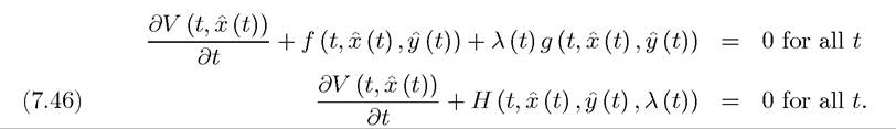
In particular, the necessary conditions can also be expressed in the form of the so-called Hamilton-Jacobi-Bellman (HJB) equation.Theorem 7.10. (Hamilton-Jacobi-Bellman Equations) Let V (t, x) be as defined
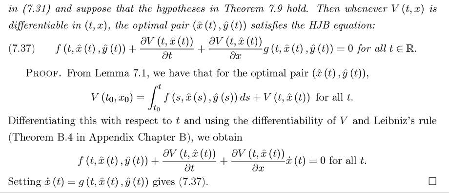
The HJB equation will be useful in providing an intuition for the Maximum Principle, in the proof of Theorem 7.9 and also in many of the endogenous technology models studied below. For now it suffices to note a few important features. First, given that the continuous differentiability of f and g, the assumption that V (t, x) is differentiable is not very restrictive, since the optimal control y(t) is piecewise continuous. From the definition (7.31), at all t where y (t) is continuous, V (t, x) will also be differentiable in t. Moreover, an envelope theorem type argument also implies that when y (t) is continuous, V (t, x) should also be differentiable in x (though the exact conditions to ensure differentiability in x are somewhat involved). Second, (7.37) is a partial differential equation, since it features the derivative of 277
V with respect to both time and the state variable x. Third, this partial differential equation also has a similarity to the Euler equation derived in the context of discrete time dynamic programming. In particular, the simplest Euler equation (6.22) required the current gain from increasing the control variable to be equal to the discounted loss of value. The current equation has a similar interpretation, with the first term corresponding to the current gain and the last term to the potential discounted loss of value. The second term results from the fact that the maximized value can also change over time.
Since in Theorem 7.9 there is no boundary condition similar to x (tι) = xι, we may expect that there should be a transversality condition similar to the condition that λ (t1) = 0 in Theorem 7.1. One might be tempted to impose a transversality condition of the form
(7.38) 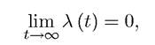
which would be generalizing the condition that λ (t1) = 0 in Theorem 7.1.
But this is not in general the case. We will see an example where this does not apply soon. A milder transversality condition of the form(7.39) 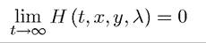
always applies, but is not easy to check. Stronger transversality conditions apply when we put more structure on the problem. We will discuss these issues in Section 7.4 below. Before presenting these results, there are immediate generalizations of the sufficiency theorems to this case.
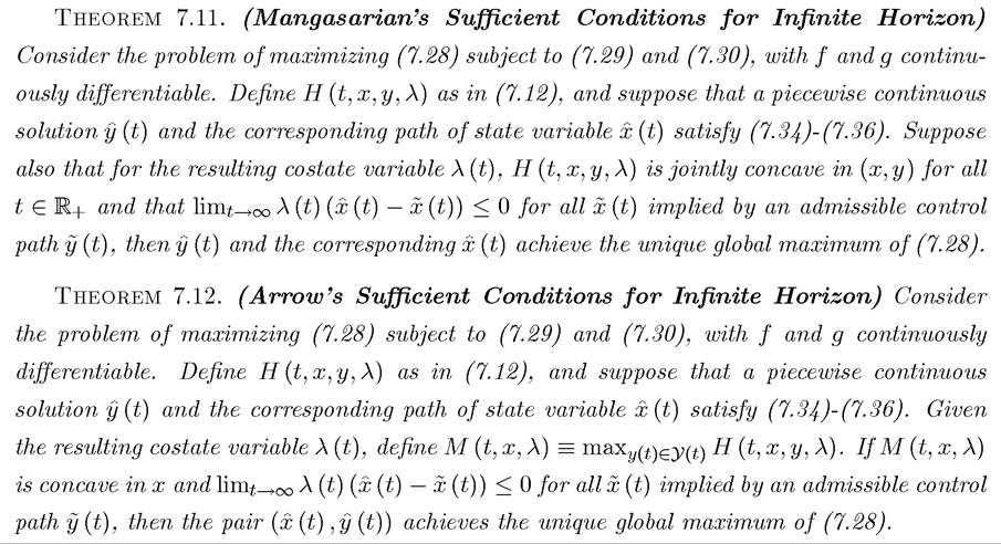
The proofs of both of these theorems are similar to that of Theorem 7.5 and are left for the reader (See Exercise 7.11). Since x (t) can potentially grow without bounds and we require 278
only concavity (not strict concavity), Theorems 7.11 and 7.12 can be applied to models with constant returns and endogenous growth, thus will be particularly useful in later chapters. Notice that both of these sufficiency theorems involve the difficult to check condition that  implied by an admissible control path
 This condition will disappear when we can impose a proper transversality condition.
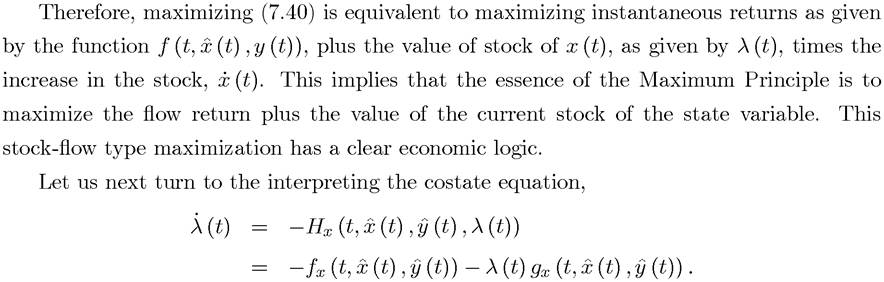
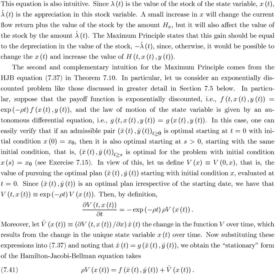
7.3.2. Economic Intuition. The Maximum Principle is not only a powerful mathematical tool, but from an economic point of view, it is the right tool, because it captures the essential economic intuition of dynamic economic problems. In this subsection, we provide two different and complementary economic intuitions for the Maximum Principle. One of them is based on the original form as stated in Theorem 7.3 or Theorem 7.9, while the other is based on the dynamic programming (HJB) version provided in Theorem 7.10.
To obtain the first intuition consider the problem of maximizing

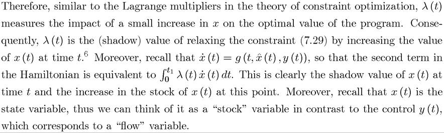
6Here I am using the language of “relaxing the constraint” implicitly presuming that a high value of x (t) contributes to increasing the value of the objective function. This simplifies terminology, but is not necessary for any of the arguments, since λ (t) can be negative.
This is a very important and widely used equation in dynamic economic analysis and can be interpreted as a “no-arbitrage asset value equation,” and given its importance, an alternative 280
derivation is provided in Exercise 7.16. Intuitively, we can think of V as the value of an asset traded in the stock market and ρ as the required rate of return for (a large number of) investors. When will investors be happy to hold this asset? Loosely speaking, they will do so when the asset pays out at least the required rate of return. In contrast, if the asset pays out more than the required rate of return, there would be excess demand for it from the investors until its value adjusts so that its rate of return becomes equal to the required rate of return. Therefore, we can think of the return on this asset in “equilibrium” being equal to the required rate of return, ρ. The return on the assets come from two sources: first, “dividends,” that is current returns paid out to investors. In the current context, this corresponds to the flow payoff If this dividend were constant and equal to d,
and there were no other returns, then we would naturally have that
However, in general the returns to the holding an asset come not only from dividends but also from capital gains or losses (appreciation or depreciation of the asset). In the current context, this is equal to Therefore, instead of ρV = d, we have
Thus, at an intuitive level, the Maximum Principle amounts to requiring that the maximized value of dynamic maximization program, V (x (t)), and its rate of change, , should be consistent with this no-arbitrage condition.
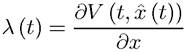
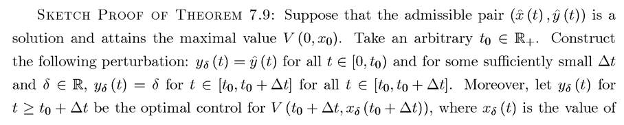
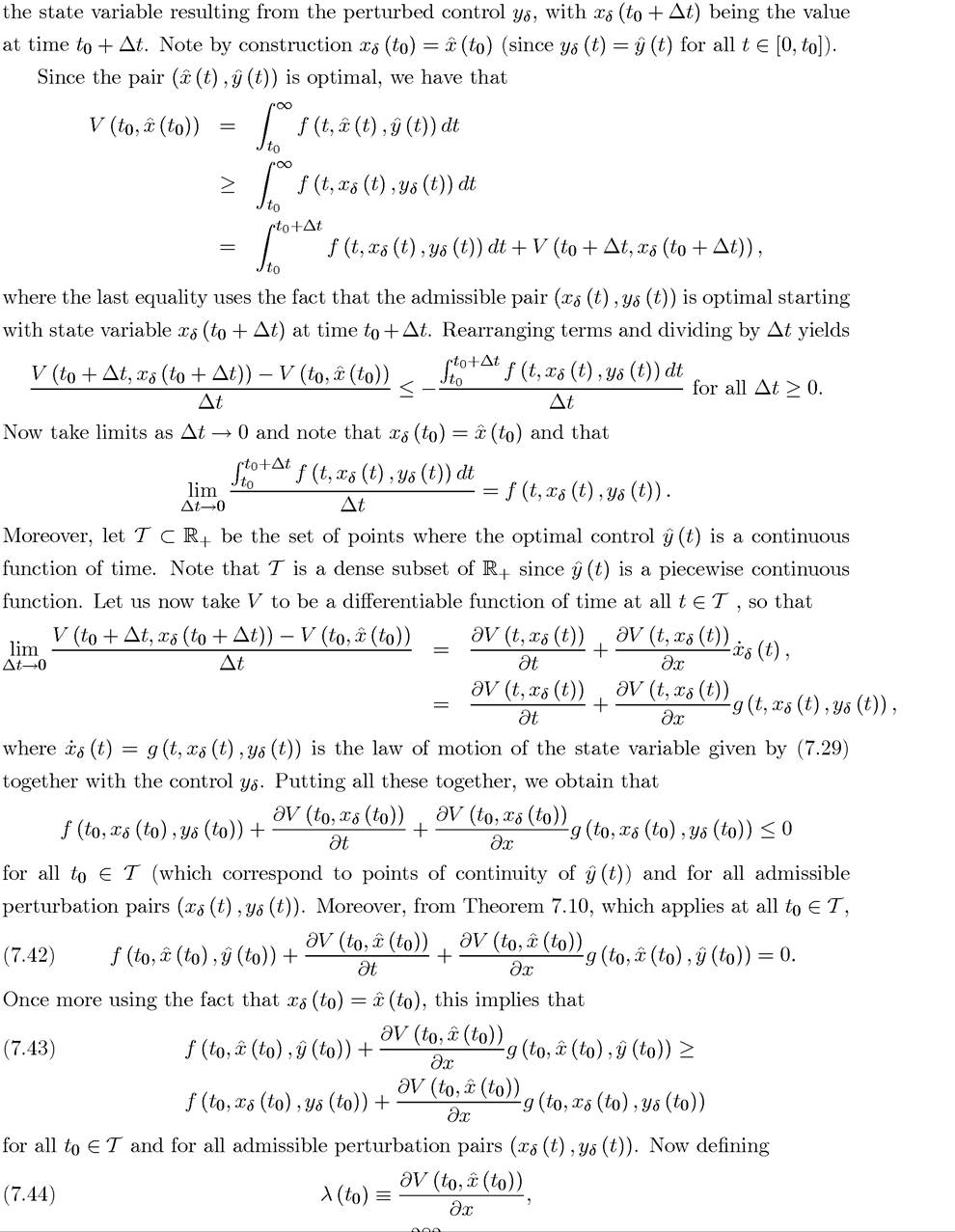
7.3.3. Proof of Theorem 7.9*. In this subsection, we provide a sketch of the proof of Theorems 7.9. A fully rigorous proof of Theorem 7.9 is quite long and involved. It can be found in a number of sources mentioned in the references below. The version provided here contains all the basic ideas, but is stated under the assumption that V (t, x^) is twice differentiable in t and x. As discussed above, the assumption that V (t, x) is differentiable in t and x is not particularly restrictive, though the additional assumption that it is twice differentiable is quite stringent.
The main idea of the proof is due to Pontryagin and co-authors. Instead of smooth variations from the optimal pair the method of proof considers “needle-like”
variations, that is, piecewise continuous paths for the control variable that can deviate from the optimal control path by an arbitrary amount for a small interval of time.
281
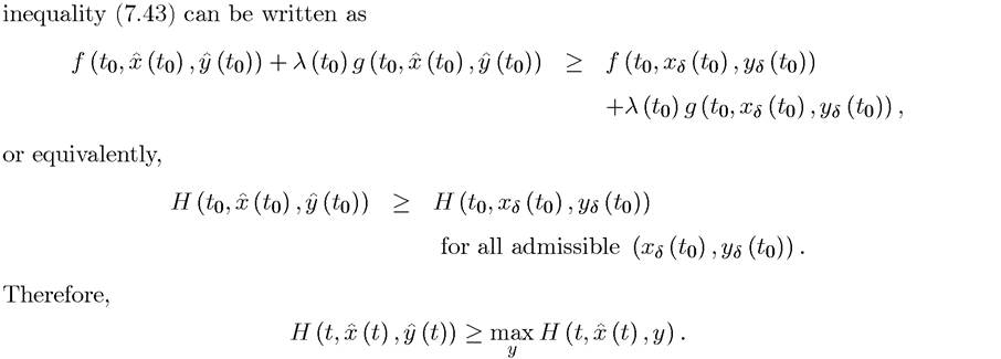
This establishes the Maximum Principle.
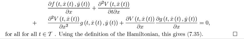
The necessary condition (7.34) directly follows from the Maximum Principle together with the fact that H is differentiable in x and y (a consequence of the fact that f and g are differentiable in x and y). Condition (7.36) holds by definition. Finally, (7.35) follows from differentiating (7.42) with respect to x at all points of continuity of y (t), which gives
7.4. More on Transversality Conditions
We next turn to a study of the boundary conditions at infinity in infinite-horizon maximization problems. As in the discrete time optimization problems, these limiting boundary conditions are referred to as “transversality conditions”. As mentioned above, a natural conjecture might be that, as in the finite-horizon case, the transversality condition should be similar to that in Theorem 7.1, with tι replaced with the limit
The following example, which is very close to the original Ramsey model, illustrates that this is not the case; without further assumptions, the valid transversality condition is given by the weaker condition (7.39).
Example 7.2. Consider the following problem:
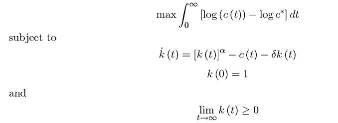
 In other words,
 is the maximum level of consumption that can be achieved in the steady state of this model and
 is the corresponding steady-state level of capital. This way of writing the objective function makes sure that the integral converges and takes a finite value (since c (t) cannot exceed c* forever).
The Hamiltonian is straightforward to construct; it does not explicitly depend on time and takes the form

and implies the following necessary conditions (dropping time dependence to simplify the notation):
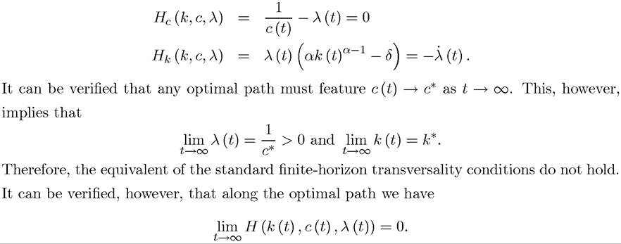
We will next see that this is indeed the relevant transversality condition.
Theorem 7.13. (Transversality Condition for Infinite-Horizon Problems) Suppose that problem of maximizing (7.28) subject to (7.29) and (7.30), with f and g continuously differentiable, has an interior piecewise continuous solution with corresponding path of state variable x(t). Suppose moreover that
 exists (where
 is de
is de
fined in (7.33)). Let H (t,x,y,λ) be given by (7.12). Then the optimal control and the corresponding path of the state variable X(t) satisfy the necessary conditions (7.34)-(7.36) and the transversality condition

Proof. Let us focus on points where V (t, x) is differentiable in t and x so that the Hamilton-Jacobi-Bellman equation, (7.37) holds. Noting that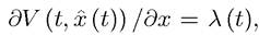 this
this
equation can be written as
284
7.5.