Distributional Conflict and Economic Growth in a Simple Society

The discussion in the previous section illustrated the complex set of forces that might affect collective choices concerning economic institutions and policies. The rest of this chapter and the next will focus on various dimensions of social conflict that will make societies adopt different economic institutions and policies, leading to different growth trajectories.

While my ultimate purpose is to present a relatively comprehensive framework, it is useful to start with a minimalist setup. For this reason, in this and the next two sections, I will discuss the implications of distributional conflict for economic growth in a simple society, in which individuals are permanently allocated to certain groups (such as producers, landowners, workers) and the main distributional conflict is among groups. The latter feature is ensured by assuming that individuals within each group are ex ante identical and by restricting the set of fiscal instruments such that it is not possible to redistribute resources from one member of the group to another (at least not along the equilibrium path). The former feature, on the other hand, rules out issues of occupational choice and social mobility, which will be discussed in the next chapter. The main advantage of a simple society for our purposes here is that, thanks for the combination of a limited set of fiscal instruments and the symmetry of individuals within social groups, it enables a tractable aggregation of political preferences of individuals. We will analyze models in which there is a non-degenerate distribution of endowments (e.g., wealth) across individuals, such as the canonical political economy model, in Section 22.7 below. While these models would be significantly richer than the simple society studied here, the economic forces that shape the political economy equilibrium will be similar, which motivates my choice of presenting a detailed analysis of political economy equilibrium in a simple society in the next few sections.

Consider a model in which there are three groups of individuals. The first is workers who supply their labor inelstically. The second group consists of entrepreneurs who have access to a production technology and make the investment decisions. The third group is the elite who make the political decisions. In particular, below I will assume that the political system is an oligarchy, dominated by the elite. The assumption that the elite make the political decisions, while the most important economic decisions, the level of investment, are 938

made by entrepreneurs will highlight the impact of distributional conflict (given the set of fiscal instruments) on equilibrium policies and production in the sharpest possible way. The presence of three groups is important for the modeling of the effect of competition between the elite and other producers in the labor market in Sections 22.3 and 22.4. The model will then be enriched in various different ways in this and the next chapter by introducing additional heterogeneity, incorporating occupational choice, and also endogenizing the distribution of political power among the various members of the society.

The baseline model is designed to be as similar to the standard neoclassical model in discrete time studied in Chapters 6 and 8 as possible. The focus on the neoclassical growth model was justified above (so as to abstract from imperfections other than those due to the political economy interactions). The focus on discrete time facilitates both the exposition and the analysis of game-theoretic interactions that are inherent in political-economy situations.

22.2.1. The Basic Environment. The economy is populated by a continuum 1 + θ^e + θ^m of risk neutral agents, each with a discount factor equal to β < 1. There is a unique non-storable final good denoted by Y. The expected utility of agent i at time 0 is given by: where Ci (t) ∈ R denotes the consumption of agent i at time t and E_t is the expectations operator conditional on information available at time t.

There is a continuum of workers, with measure normalized to 1, who supply their labor inelastically. The elite, denoted by e, initially hold political power in this society. There is a total of θ^e elites. As a starting assumption, we suppose that the elite do not take part in productive activities. Political economy interactions become considerably richer and more interesting (but also somewhat more involved) when the elite are also competing with other groups in product or factor markets. This issue will be discussed in Section 22.3. Finally, there are θ^m “middle class” agents, denoted by m, who are the entrepreneurs in the economy with access to the production technology. The label of “middle class” for the entrepreneurs is motivated by some historical examples that will be discussed in the next chapter and plays no role in the formal analysis. The sets of elite and middle class producers are denoted by S^e and S^m respectively. With a slight abuse of notation, I will use i to denote either individual 939

or group (though when referring to groups, I will use i as superscript, and when referring to individuals, as subscript). The identity of the agents (their social group membership) does not change over time.

Each entrepreneur (middle-class agent) i ∈ S^m has access to the following production technology for producing the final good:

where Yi (t) is final output produced by entrepreneur i, Ki (t) and Li (t) are the total amount of capital and labor he uses in production.

with Li (t) ≤ L. As in the standard neoclassical model, we assume that a fraction δ of capital depreciates.

The equilibrium of this economy without “political economy” is straightforward. Imagine that there are no taxes and labor markets are competitive. Let k ? K/L denote the capital­labor ratio as usual and f (k) be the per capita production function again defined as usual (i.e., f (k) ? F (K/L, 1)). This immediately implies that each entrepreneur will choose the capital-labor ratio given by

for each t, whereis the inverse of the marginal product of capital (the derivative

of the f function). Equation (22.4) is identical to the standard steady-state equilibrium condition from Chapters 6 and 8, which equates the gross marginal product of capital in steady statewith the inverse of the discount factor, β^-1 (for example, recall

equation (6.38) in Chapter 6).

that there are no transitional dynamics; irrespective of initial conditions, each entrepreneur will immediately choose the capital-labor ratio k* as in (22.4).

Another special feature of this economy is that it may fail to achieve full employment. Recall that the total labor force is equal to 1. However, equation (22.5) shows that the level of employment of each employer may be strictly less thanbecause of the maximum size constraint on firms. When this is the case,workers will be unemployed and

wages will be equal to 0. When there is excess supply of labor, each entrepreneur i ∈ S^m will employ L workers and total employment will fall short of the total supply. When there is no excess supply, the entire labor force will be employed and the allocation of these workers across the entrepreneurs is arbitrary (since all entrepreneurs would be making zero profits). To simplify the exposition, I assume, without loss of any generality, that even in this case, all

entrepreneurs will employ the same number workers, so that the equilibrium labor allocation

In addition, in this section I assume that

which insures that there will be full employment and thusUnder this assumption,

the equilibrium wage rate at every date will also be given by the usual expression (which follows from Theorem 2.1 in Chapter 2)

where k^* is given in (22.4) above.

22.2.2. Policies and Economic Equilibrium. Before we can characterize political equilibria, we need to specify the set of available fiscal instruments (policies), and then define an economic equilibrium for given sequences of policies. Different economic equilibria will involve different levels of welfare for different agents, thus implicitly defining induced pref­erences over the policies and economic institutions leading to different economic equilibria (this point is further discussed in the next chapter). The political equilibrium then aggre­gates these preferences over different sequences of policies, taking into account the economic equilibrium that they will induce, to arrive to collective choices. In the current model, this last step is simplified given our focus on sequences of policies that maximize the utility of the elite. The characterization of the economic equilibrium is, in turn, much simplified thanks to linear preferences. Nevertheless, it is useful to go through each of these steps in order.

As for policies, we assume that the society has access to four different policy instruments at each date t:

Notice that we have assumed the lump-sum transfers are nonnegative. This rules out lump-sum taxes that could raise revenues without creating distortions. Instead revenues can only be raised using the linear tax on output, which, as we will see, will be distortionary. While lump-sum taxes might sometimes be possible, the ability of individuals to move into the informal sector or stop working puts limits on the use of lump-sum taxes. Nevertheless, the restriction to a simple linear tax rate is quite restrictive and there might often exist more efficient ways of raising revenues. In political economy models such restrictions are sometimes made so as to be able to characterize the equilibrium (for example, when using the Median Voter Theorem, see Section 22.6). Here we are imposing these restrictions to emphasize how the interaction between the decoupling of political and economic power and a limited menu of fiscal instruments can lead to distortionary policies. We will return to the question of why, even with efficient means of raising revenues, political economy motives can lead to non-growth-enhancing policies (see Section 22.4).

We also need to specify the timing of events within each date, and especially we have to be specific about when taxes are set (and this is the main reason why discrete time models are slightly more convenient in this context). We assume that there is one period commitment to taxes. In other words, the timing of events is such that at each t, we start with a pre-determined tax rate on output τ (t), as well as the capital stocks [Ki (t)]i∈sm of the entrepreneurs. Then entrepreneurs decide how much labor to hire(and in

the process the labor market clears). Output is produced and a fraction τ (t) of the output is collected as tax revenue. After the tax revenue is observed, the political process (for example the politically powerful elite) decides the transfers, subject to the government budget constraint

where the left-hand side denotes total government expenditure in transfers and the right-hand side is the pre-determined tax rate times the output of all entrepreneurs. Next, the political

process announces the tax rate τ (t + 1) that will apply at the next date and entrepreneurs, after observing this tax rate, choose their capital stocks for the next date,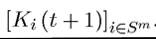

The important feature in this timing of events is that entrepreneurs know exactly what tax rate they will face when choosing their capital stock. The alternative, where the capital stock is chosen before the tax rate, will be discussed in Section 22.3. For now it suffices to say that this alternative will lead to greater distortions because of holdup problems. It is therefore more natural to start with the timing of events specified here.

Let us also denote the policy or tax sequence starting at time t by

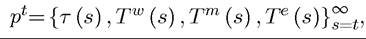which specifies a feasible infinite sequence of policies starting at time t. One has to be a little careful about feasibility here, because whether a policy sequence is feasible or not cannot be determined without reference to the actions of the entrepreneurs (for example, any policy sequence with positive transfers cannot be feasible if all entrepreneurs choose zero capital stock). For our purposes, this is not important, since with linear preferences, only the tax rate sequence matters for capital and production decisions, and the transfers can be determined as residuals to satisfy the government budget constraint (22.8). It should nonetheless be noted that each individual, in particular, each entrepreneur, is infinitesimal, thus ignores his impact on total tax revenues and on the government budget constraint.

We can now define an economic equilibrium from time t onwards given a pre-determined distribution of capital stock among the entrepreneurs, [Ki (f)]_i∈_sm and a feasible policy se-

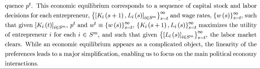
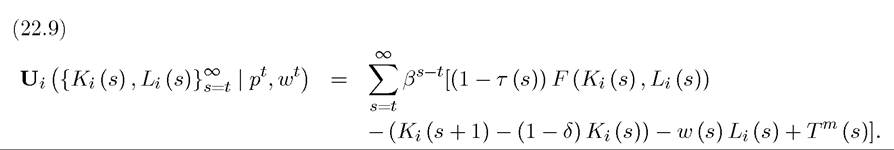
Since workers supply labor inelastically, the only nontrivial decisions are by the entrepre­neurs. As a first step towards characterizing the equilibrium, note that given any feasible policy sequence p^t and equilibrium wages w^t, the utility of an entrepreneur starting with capital stock Ki (t) at time t as a function of these policies can be written as

943

This expression makes use of the fact that preferences are linear, thus the value of the entrepreneur can be written simply in terms of the discounted sum of his consumption. His consumption, on the other hand, is simply given by the term in square brackets, since output is taxed at the rate τ (t) at time t and moreover, a fraction (1 — δ) of last period’s capital stock is left, so an additional investment of (Ki (t + 1) — (1 — δ) Ki (t)) is made for next period. Finally, the labor costs at the current wage are subtracted and the lump-sum transfer to middle-class entrepreneurs is added. A special feature concerning (22.9) should be noted. It is formulated for a given sequence of policies p^t. Loosely speaking, this could be thought of as the case if the sequence of policies were specified and committed to at some date. Although we are interested in political economy equilibria, where there is no commitment to future policies, we can think of the sequence of policies p^t as given from the viewpoint of an individual entrepreneur. Nevertheless, this way of writing the maximization problem of the entrepreneur does not give information about how he would react if the political process (here the elite) deviated from p^t, since this might also be associated with a change in the remainder of the policy sequence. Nevertheless, linear preferences again ensure that we do not need to worry about this issue, since, as we will see momentarily, entrepreneurial decisions will only depend on current taxes. This issue of off-the-equilibrium path behavior becomes important when preferences are not linear and will be discussed in the next section.

Maximizing (22.9) with respect to the sequences of capital stock and labor choices, we obtain the following simple first-order condition:

where ki (t + 1) denotes the capital-labor ratio chosen by entrepreneur i for time t + 1 given the tax rate τ (t + 1), which has already been announced (and committed to) at the time of the investment decision. Thanks to the Inada conditions in Assumption 2, this first-order condition holds as equality for any τ (t + 1) ∈ [0,1) and Exercise 22.1 shows that there will never be 100% taxation. Thus we do not need to spell out complementary slackness conditions.

id="Picutre 2947" class="lazyload" data-src="/files/uch_group77/uch_pgroup317/uch_uch7364/image/image2945.jpg">

It can be verified easily that if all taxes were equal to zero, i.e., τ (t) = 0 for all t, the unique solution to (22.10) would be identical to the steady-state capital-labor ratio k* in (22.4) given in the previous subsection. Naturally, when there are positive taxes, the level of capital-labor ratio will be less than k* (this follows immediately since f (∙) is strictly concave; see (22.12) below). It is also worth noting that while in the equilibrium “without political economy” (i.e., without taxes and transfers) the capital stock exhibited no transitional dynamics and 944

immediately jumped to its state-state value, this may no longer be the case in an economic equilibrium given the policy sequence p^t, since the policy sequence may involve time-varying taxes.

The most noteworthy feature of the equilibrium capital-labor ratio given in (22.10) is that, thanks to linear preferences, the choice of the capital-labor ratio by each entrepreneur at time t + 1 only depends on the tax rate τ (t + 1), and not on future taxes. We can therefore write the equilibrium capital-labor ratio at time t for all entrepreneurs as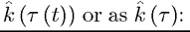

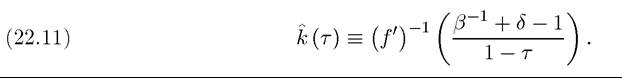
The fact that the equilibrium capital-labor ratio depends only on one tax rate and is the same for all entrepreneurs will simplify the analysis of political economy considerably. For future reference, note also that since F (∙, ∙), and thus f (∙), is twice continuously differentiable, k (τ) is also differentiable, with derivative

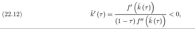
which follows by directly differentiating (22.11) and is negative in view of the fact that f⁰ (k) > 0 and f⁰⁰ (k) < 0 for all k (from Assumption 1).

Given the expression for the equilibrium capital-labor ratio in (22.11) and full employment as implied by (22.6), the equilibrium wage at time t is given by the usual expression:

which is similar to (22.7) except for the presence of the tax rate in the front.

While (22.11) gives a very simple expression for the capital stock as a function of the tax rate, without knowing more about the sequence of policies we cannot ascertain whether the sequence of equilibrium capital stocks will converge to some steady-state value (for example, this will not be the case if taxes periodically fluctuate between different levels). Nevertheless, our analysis so far has established the following proposition:

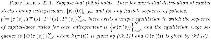
This proposition is convenient not only because the form of the equilibrium is particu­larly simple, but also because for any given sequence of policies, the aggregate equilibrium allocation is unique. If some policy sequences led to multiple equilibrium allocations, then 945

expectations concerning which of these equilibrium would be played conditional on these policy choices would complicate the analysis.^[XLIX]

22.2.3. Political Economy under Elite Control. As noted at the beginning of this section, our task of characterizing the political economy equilibrium here is considerably simplified by the assumption that political power is entirely in the hands of the elite. There is no issue of political power changing hands or the elites choosing policies in order to appease voters or other social groups. Moreover, there are no fiscal instruments that would redistribute income among the elite. Thus the political economy choices here just involve the choice of fiscal policies at each date that would maximize the net present discounted utility of a representative elite agent.

Throughout this section, we will look at the political equilibria using the notion of Markov Perfect Equilibria (MPE). This notion, which was first used in Chapter 14, requires the policy sequence p^t be such that policies dated t only depend on the dated t payoff-relevant variables (see the Appendix Chapter C for a formal definition of MPE). Here the only payoff relevant variables are the capital stocks of the entrepreneurs. Thus most generally, current policies can depend on the current distribution of capital stocks. Linear preferences again simplify the analysis, and imply that we do not need to keep track of a complicated distribution of capital stocks as the relevant state variable. Since the MPE are a subset of the Subgame Perfect Equilibria (SPE) that do not condition on past history except through payoff-relevant variables, they rule out repeated game punishments (such as those relying on trigger strate­gies). We return to a discussion of situations in which the SPE are different from the MPE below. We will also refer to the MPE in this chapter as Markov Perfect Political Economy Equilibrium.

For the characterization of the political economy choices of the elite, recall that the elite also care about their level of consumption (discounted with the discount factor β). From this observation, it is straightforward to see that they would never choose to redistribute to workers or to the middle class, thus in what follows we can restrict attention to sequences of policies that involve T^w (t) = T^m (t) = 0 for all t. Next, let us combine this fact with the government budget constraint, (22.8), which must hold as equality (since otherwise the elite could increase their consumption and utility by increasing transfers to themselves), to obtain

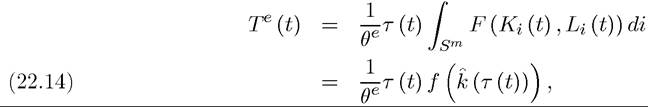
where the first line simply uses the government budget constraint (22.8), while the second line uses the equilibrium characterization in Proposition 22.1 together with the fact that with full employment, the total number of workers is equal to 1.

The problem of maximizing the utility of the elite agents can then be written as

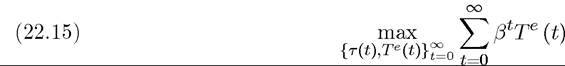
subject to (22.14) at each t. Notice again that although it appears from (22.15) as if the elite were choosing the tax sequences at date t = 0, since there is no commitment to future policies, they are in fact only setting taxes for time t + 1 at time t. But this way of writing the elite’s program will characterize the MPE since middle-class entrepreneurs capital-labor ratio decisions at time t + 1 only depend on the tax rate announced for time t + 1, and not on future or past taxes.

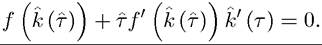
To characterize the equilibrium tax sequence, note that T^e (t) only depends on the tax rate at time t and involves the choice of the tax rate that would maximize tax revenue (i.e., that would put the elite at the peak of the “Laffer curve”) at each date. Then the utility­maximizing tax rate for the elite, ^, can be obtained as a solution to the following first-order condition:

Substituting for k' (τ) from (22.12), we obtain the following expression for T:

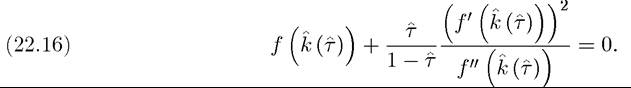
Intuitively, the utility-maximizing tax rate for the elite trades off the increase in revenues resulting from a small increase in the tax rate,, against the loss in revenues that will result because the increase in the tax rate will reduce the equilibrium capital-labor ratio, It can be verified that this tax rate T is always between 0 and 1 (see Exercise 22.1), though the maximization problem of the elite is not necessarily concave and (22.16) may have more than one solution. If this is the case, we always refer to the solution T that corresponds to a global maximum for the elite.

Notice that (22.16) implies a constant tax rate across different dates, and moreover, if we were to consider the maximization problem of the elite (22.15) after some arbitrary date t', exactly the same tax sequence would result. This is the reason why we could, without loss of

any generality, focus on the maximization problem in (22.15). We will see in the next section that this is not always the case and we need to take into account the sequential nature of the decision-making by the elite and the entrepreneurs.

This analysis so far has thus established the following characterization of the political economy equilibrium:

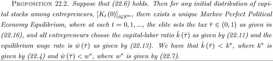
This proposition shows that a unique well-defined political equilibrium exists and involves positive taxation of entrepreneurs by the elite. Consequently, the capital-labor ratio and the wage rate are strictly lower than they would be in an economy without taxation. Strictly speaking, the equilibrium distortionary policies do not change “growth,” since we are focusing on a neoclassical economy without technological progress. As explained above, this is the only for convenience and it is straightforward to extend the framework here to incorporate endogenous growth, so that the distortionary policies do affect the equilibrium growth rate of the economy (see Exercise 22.2).

We can now return to the fundamental question raised at the beginning of this chapter: why would a society impose distortionary taxes on businesses/entrepreneurs? The model in this section gives a simple answer. Political power is in the hands of the elite, who would like to extract revenues from the entrepreneurs. Given the available tax instruments, here linear taxes on output, the only way they can achieve this is by imposing distortionary taxes. Thus the source of “inefficiencies” in this economy is the combination of revenue extraction motive by the politically powerful combined with a limited menu of fiscal instruments.

While the analysis so far shows how distortionary policies can emerge and reduce the level of investment and output below the “first-best” level, it is important to emphasize that the equilibrium here is not Pareto inefficient. In fact, given the set of fiscal instruments,the equilibrium allocation is the solution to maximizing a social welfare function that puts all the weight on the elite. Pareto inefficiency requires that, given the set of instruments and in­formational constraints, there should exist an alternative feasible allocation that would make each agent either better-off or at least as well of as they were in the initial allocation. Such an allocation can be found if we allowed lump-sum taxes. But given the restriction to linear taxes, which in the current economy are “technological,” there is no way of improving the 948

utility of the middle-class entrepreneurs and the workers without making the elite worse-off.^{[50] [51]} This is an important observation, since it implies that when we explicitly incorporate political economy aspects into the analysis, there are typically no “free lunches”—that is, no way of making all agents better-off. This is the reason why political economy considerations typi­cally involve tradeoffs between losers and winners in the process of various different changes in institutions and policies. Since the allocation in Proposition 22.2 involves distortionary policies and reduces output relative to the first-best allocation, we might want to refer to this outcome as “inefficient” (despite the fact that it is not “Pareto inefficient”). In fact, this label is often used for such allocations in the literature and I will follow this practice. When using these terms, it is important to bear in mind that such “inefficiencies” do not mean Pareto inefficiencies.

As a preliminary answer, Proposition 22.2 is a useful starting point. However, it leaves a number of important questions unanswered. First, it does not provide useful comparative statics regarding when we should expect higher rates of distortion of the taxes. Second, it takes the distribution of political power as given, and it appears important for the results that political power rests in the hands of the non-productive elite, who are using the fiscal instruments to extract resources from middle-class producers. If political power were in the hands of the middle-class entrepreneurs rather than the non-productive elite, the choice of fiscal instruments would be very different. A first intuition might be that the entrepreneurs would never tax themselves. However, Exercise 22.3 shows that this is not necessarily the case and the middle-class entrepreneurs may prefer to tax themselves as a way of indirectly changing equilibrium wages. This is important because the role of fiscal policies in changing factor prices is often underappreciated and we will argue in Section 22.3 that it is one of the more important sources of political distortions in the process of growth. Third, this analysis takes the menu of available fiscal instruments as given. If the elite had access to lump-sum taxes, it could extract revenue from the entrepreneurs without creating distortions. We will extend the current framework to provide answers to all of these questions in this and the next chapter. Before doing this, we will first consider a more specific version of the economy analyzed so far where the production function is Cobb-Douglas. This Cobb-Douglas economy, by virtue of its tractability, will be a workhorse model for our analysis in Sections 22.3 and

22.4. Finally, in Section 22.5, we will consider a generalized version of the environment here where individuals have concave preferences.

22.2.4. The Canonical Cobb-Douglas Model of Distributional Conflict. Con­sider a slightly specialized version of the economy analyzed so far, with two differences. First, the production function of each entrepreneur takes the following Cobb-Douglas form:

where Ai (t) is a labor-augmenting group-specific or individual-specific productivity term, which will be used later in this chapter. For now, we can set Ai (t) = A^m for all i ∈ S^m. The term 1/a in the front is included as a convenient normalization. We will see that the Cobb- Douglas form will enable an explicit-form characterization of the political equilibrium and will also link the elasticity of output with respect to capital to the equilibrium taxes. This is the reason why I refer to this model is the “canonical model” of distributional conflict. Second, the analysis so far has shown that with linear preferences, incomplete depreciation of capital plays no qualitative role, so I will also simplify the notation by assuming full depreciation of capital, i.e., δ = 1. This assumption is without any substantive implications.

The Cobb-Douglas production function in (22.17) implies that the per capita production function is given by

Combining this production function with the assumption that δ = 1, equation (22.10) above implies shows that at date t + 1 each entrepreneur will choose a capital-labor ratio k (t + 1) such that

The utility-maximizing tax policy of the elite is still given by equation (22.16), which com­bined with the Cobb-Douglas form here implies that the utility-maximizing tax for the elite at each date is given by

This formula is both simple and economically intuitive. When α is high, the production function is nearly linear in capital. This implies that the demand for capital as a function of its effective price is highly elastic. With such an elastic demand for capital, high taxes would lead to a large decline in the capital stock. Thus by charging high taxes, the elite would be reducing their own revenues. Put differently, with an elastic demand for capital (which in turn follows from production function that is not very concave in capital), the peak of the Laffer curve for the elite is at a low tax rate. On the other hand, if α is low, the production function is highly concave in capital, thus even a significant tax rate will not lead to a large decline in the equilibrium capital-labor ratio choice of the entrepreneurs. In this case, the elite will find it profitable to charge very high taxes.

Both the tractability afforded by the Cobb-Douglas production function and the link between the concavity of the production function and equilibrium taxes that it highlights make this a very useful framework, which we will next use in a number of applications below.

22.3.