Dynamic Simulations of a Calibrated Ramsey Model

To gain a better insight into the quantitative aspects of the process of adjustment in the Ramsey model, we can use numerical simulations for specific values of the parameters of the model.

4.5.1 The Ramsey Model in Discrete Time

Instead of assuming that time is a continuous variable, time is now measured as successive time periods, where t = 0, 1, 2, …. The variable x_t indicates the variable x in period t. Population and the efficiency of labor grow at constant exogenous rates n and g per period, respectively. Thus, we have

The intertemporal utility function of the representative household in given by

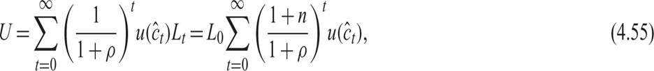
where ĉ is per capita consumption.

We assume, as in the continuous time case, that the single-period utility function u has the form of the constant elasticity of intertemporal substitution utility function:

With this assumption, after expressing consumption per efficiency unit of labor c, we get

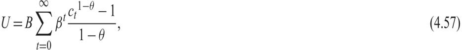
where B = h₀^1−θL₀, and .

We thus assume that the representative household maximizes (4.57) under the sequence of constraints (4.58). The Lagrange function for this problem is given by

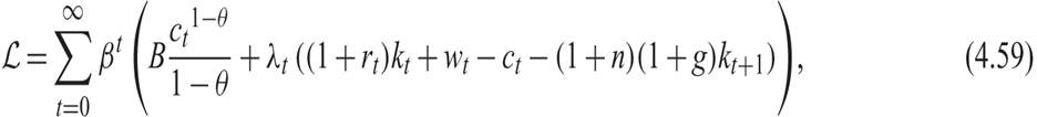
where λ_t is the sequence of Lagrange multipliers. The first-order conditions for the maximization of (4.59) are given by

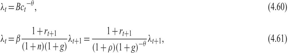
Combining (4.60) and (4.61), we get

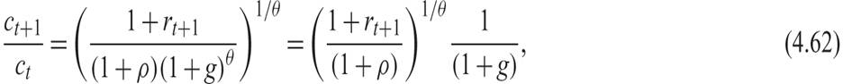
which is the Euler equation for consumption in the discrete-time Ramsey model.

Assuming a competitive capital market, the real interest rate will be given by

and substituting (4.63) into (4.62), we get

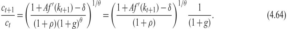
As a result, the balanced growth path c_t+1 = c_t = c^* requires a capital stock k^*, the marginal product of which satisfies

To calculate equilibrium consumption, we utilize the capital accumulation equation (4.58). After substituting for the real interest rate and the real wage, this constraint can be expressed as

In the steady state (balanced growth path), we have

which determines steady state consumption, in the sense that savings are equal to the equilibrium investment that maintains the capital stock at its steady state value k^*.

The dynamic adjustment toward this steady state is described by the system of nonlinear difference equations (4.64) and (4.66).

4.5.2 The Calibrated Ramsey Model

To simulate the model numerically, we assume, as in the case of the simulations of the Solow model, that the production function is Cobb-Douglas of the form

where A > 0 is total factor productivity, 0 < α < 1 is the exponent (share) of capital in the production function, and 1 − α is the exponent of labor.

The real interest rate and the real wage per efficiency unit of labor are given by the marginal productivity conditions

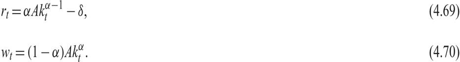
The pair of nonlinear adjustment equations for capital and consumption per efficiency unit of labor are obtained by adapting (4.64) and (4.66) for the Cobb-Douglas production function:

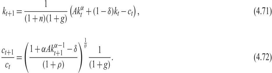
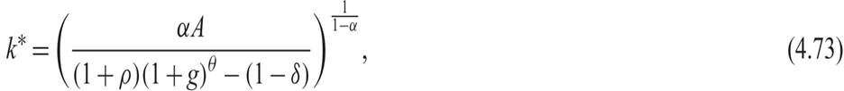
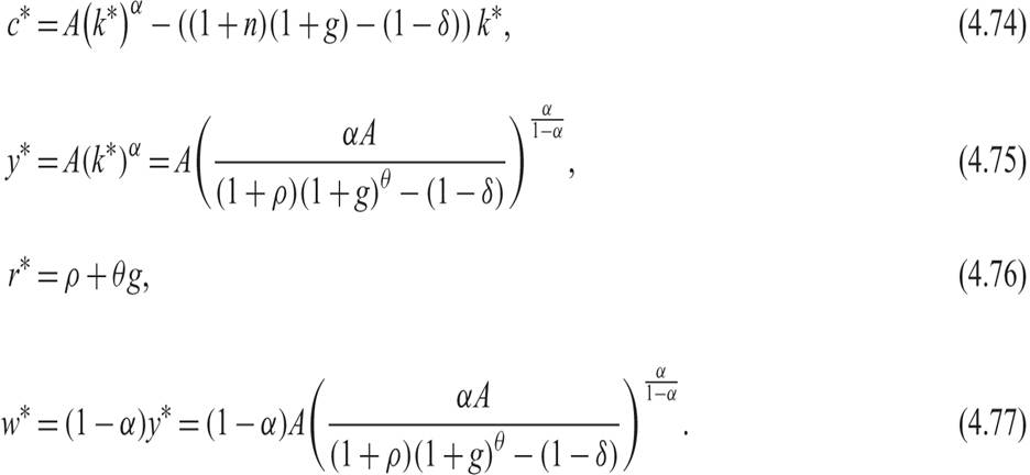
The steady state values for the capital stock, output, consumption, real wages, and the real interest rate can be calculated by setting c_t = c_t+1 = c^* and k_t = k_t+1 = k^* in (4.71) and (4.72), and using (4.68), (4.69), and (4.70) to calculate output, the real interest rate, and the real wage:

From (4.73) and (4.75), note that the rate of growth of population does not affect the steady state capital stock and steady state output and income. This is because the representative household internalizes the welfare of future generations in its optimal savings decision.

From (4.74) and (4.75), the steady state savings rate is equal to

The optimal steady state savings rate will be a positive function of the rate of growth of population. It will also be smaller than the share of capital α, assuming that we have chosen the discount factor of the representative household to be smaller than unity:

Simulating the system of the two nonlinear difference equations (4.71) and (4.72) numerically for specific values of the parameters, we can calculate the dynamic adjustment of capital and consumption toward the balanced growth path. The dynamic adjustment of the other variables can then be calculated from (4.68), (4.69), and (4.70).

4.5.3 Dynamic Simulations of the Model

The parameter values used in the simulations are as follows: A = 1, α = 0.333, ρ = 0.02, θ = 1, n = 0.01, g = 0.02, δ = 0.03. These values are consistent with the values that we used in the simulations of the Solow model and those used to calculate the speed of adjustment of both models.

As in the case of the Solow model, we consider two alternative scenarios: a permanent drop in the pure rate of time preference of the representative household ρ by 1% (from 0.02 to 0.019), and a permanent increase in total factor productivity A by 1% (from 1 to 1.01). The results of the simulations are presented in figures 4.6 and 4.7.

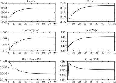
Figure 4.6 Impulse response functions of the calibrated Ramsey model for a 1% permanent drop in the pure rate of time preference.

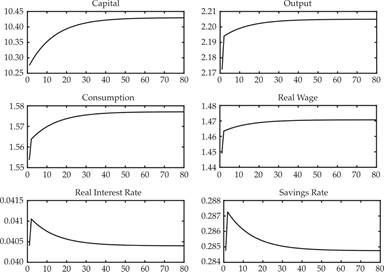
Figure 4.7 Impulse response functions of the calibrated Ramsey model for a 1% permanent increase in total factor productivity.

In the simulation of figure 4.6, the economy is on its original balanced growth path, and after period 1, the pure rate of time preference of the representative household ρ falls permanently and unexpectedly by 1%, from 0.02 to 0.019. This leads directly to a drop in consumption, a rise in the savings rate, a gradual accumulation of physical capital, a gradual increase in output and real wages, and a gradual decline in the real interest rate. The reason for rising real wages is the gradual increase of the marginal product of labor caused by the accumulation of capital. The reason for the declining real interest rate is that the marginal product of capital gradually declines because of the accumulation of capital. The economy gradually converges to a new balanced growth path. On the new balanced growth path, capital per efficiency unit of labor is higher by around 0.4%, output and real wages by 0.15%, consumption by 0.03% (due to the decline in the savings rate). The real interest rate has declined by 0.01 percentage points, the same as the increase in the pure rate of time preference. The steady state savings rate rises slightly, from 28.5% to 28.6%.

In the simulation of figure 4.7, the economy is initially on its original balanced growth path. After period 1, total factor productivity A rates rises permanently and unexpectedly by 1%, from 1 to 1.01. This increase leads to an immediate increase in production, consumption, savings, and the marginal product of both labor (the real wage) and capital (the real interest rate). The increase in savings causes a gradual accumulation of capital, which leads to a further gradual increase in production, consumption, and the real wage, but a gradual fall in real interest rates. The reason for the falling real interest rate is the gradual reduction of the marginal product of capital caused by the accumulation of capital. The economy gradually converges to a new balanced growth path. On this path, capital per efficiency unit of labor has increased by about 1.5%; output, consumption, and real wages are also higher by 1.5%; and the real interest rate has returned to its original equilibrium. The steady state real interest rate only depends on the pure rate of time preference of the representative household, the elasticity of intertemporal substitution, and the rate of technical progress. The increase in total factor productivity by 1% leads to an increase in real income by 1.5% (i.e., more than 1%) because the increase in total factor productivity causes a temporary rise in the savings rate and accumulation of capital, which in turn induces additional increases in real incomes and consumption. As can be seen from the steady state equation for output (4.75), the elasticity of steady state output with respect to total factor productivity is equal to 1/(1 − α) > 1.

4.6