Properties of the Adjustment Path and the Speed of Convergence

To algebraically analyze the convergence of the economy toward the balanced growth path, let us replace the pair of nonlinear differential equations (4.20) and (4.29) with linear approximations around the balanced growth path.

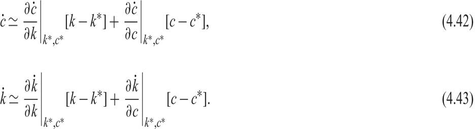
The system of linear differential equations (4.42) and (4.43) can be written as

where = c − c*, and = k − k*.

From (4.29), we have

Using (4.46) to evaluate the derivatives in (4.44), we get

Correspondingly, from (4.20), we have

and using (4.48) to evaluate the derivatives in (4.45), we get

where β = ρ − n − (1 − θ)g.

With two simple divisions on each side of (4.47) and (4.49), we can re-write them as

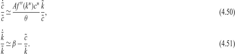
Expressions (4.50) and (4.51) imply that the rates of change of the distance of consumption and the capital stock from their steady state values depend only on the ratio of their respective distances from their steady state values.

The roots of the system of differential equations (4.47) and (4.49) are determined by

Only the negative root leads the system to the balanced growth path. We thus have that

Assuming a Cobb-Douglas production function of the form Af(k) = Ak^α, (4.53) can be written as

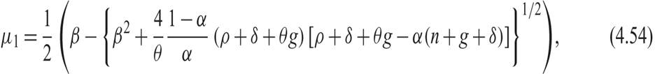
where α is the exponent of capital in the Cobb-Douglas production function.

Equation (4.54) expresses the speed of adjustment of the economy toward the balanced growth path as a function of structural parameters related to the preferences of the representative household, the technology of production, population growth, the rate of technical progress, and the depreciation rate of the capital stock.

To get a quantitative feel for the speed of adjustment, let us assume, as in the Solow model, that α = 1/3. Let us also assume that θ = 1 and that, per year, ρ = 2%, n = 1%, g = 2%, δ = 3%. The assumption about θ implies logarithmic preferences. With these assumptions, the annual real interest rate on the balanced growth path is equal to 4%, and the savings rate on the balanced growth path is 28.5%. And β turns out to be 1% per year.

Using these parameter values and equation (4.54), the speed of adjustment toward the balanced growth path turns out to be −7.9% per year. The half-life of the adjustment process (i.e., the time it takes to cover half the distance between any initial position and the balanced growth path) is 8.8 years. With the same assumptions about parameters, the speed of adjustment in the Solow model is −4% per year, and the half-life of the adjustment process is 17.3 years.

Adjustment in the representative household model is thus faster than in the corresponding Solow model for similar parameter values.

Apart from the fact that savings behavior is optimal in the Ramsey model, this model in other respects has the same theoretical weaknesses as the Solow model. The rate of technical progress, which determines long-run growth in per capita output, income, real wages, consumption, and the capital stock is exogenously given rather than determined by the model.

As with the Solow model, what the Ramsey model does explain is the level (not the growth rate) of per capita output, income, real wages, consumption, and the capital stock on the balanced growth path. It also explains the adjustment process toward the balanced growth path.

4.5