Money and the Price Level in Dynamic General Equilibrium Models

To shed further light on the determinants of money demand, the role of money, and also the long-run neutrality of money, let us analyze a series of alternative dynamic and dynamic stochastic general equilibrium models, in which prices are flexible and the demand for money results from the optimizing behavior of households and firms.

As we shall see, the long-run neutrality of money is a property that characterizes all the models examined, although these models have different properties regarding the role of money and the operation of the money market, the determination of the price level, the liquidity effect, and the implications of interest rate rules.

12.6.1 The Samuelson OLG Model

We start with a simple version of the OLG model of Samuelson [1958], in which the demand for money arises solely from its role as a store of value.

Assume that the economy consists of successive generations of households, each of which lives for two periods. Every household has exogenous income Y₁ in the first period of life and Y₂ in the second period. This income is in the form of a perishable good that cannot be transferred from period to period. The only nonperishable commodity is money, which can be used as a store of value. Normalize the size of each generation to 1 and abstract from population growth, assuming it is equal to zero.

The utility function of the household in the generation born at time t depends on the consumption of goods in the first and second periods of life. Consequently, the household born in period t maximizes the utility function

under the constraints

C₁ is household consumption in the first period; C₂ is consumption in the second period; u is a concave utility function; and β = 1/(1 + ρ) is the discount factor, where ρ is the pure rate of time preference.

Assume for simplicity that the household utility function is logarithmic and takes the form

From the maximization of (12.10) under the constraints (12.8) and (12.9) it follows that the consumption of the young in period t is determined by

The old generation in period t (those who are in their second period of life) consumes all its current income, plus its savings (i.e., the quantity of money carried over from the previous period):

The equilibrium condition in the goods market implies that

From (12.11)–(12.13) it thus follows that

Solving (12.14) for the demand for real money balances yields

From (12.15), it follows that, if there exists a constant equilibrium price level P^*, it should satisfy

The condition for a positive equilibrium price level, and thus a positive demand for real money balances, is that

The demand for money, and hence the price level, will be positive only if the discounted first-period income of households exceeds the second-period income.

In the Samuelson model, money improves welfare, because it allows households to engage in intertemporal trade and smooth consumption over time. In the absence of money, consumption in each period would have to be equal to current income for all generations. Such an equilibrium would be clearly suboptimal compared to the equilibrium of a monetary economy that allows for consumption smoothing.

To examine the dynamic adjustment of the price level, we can substitute (12.16) in (12.14). The resulting adjustment equation for the price level takes the form

Because the price level is a non-predetermined variable, the condition for the stability of the dynamic adjustment to the equilibrium price level P^* is (12.17) (i.e., that the root of the difference equation (12.18) is greater than one). Consequently, the condition for the existence of a positive equilibrium price level coincides with the condition for the stability of the equilibrium. If (12.17) is satisfied, then a positive equilibrium price level exists. In addition, the equilibrium is a saddle point (i.e., dynamically stable).

The Samuelson OLG model is one of the simplest dynamic general equilibrium models that generates a positive demand for money as a store of value. The neutrality of money follows immediately. From equation (12.16), an increase in the money supply M will cause an increase in the equilibrium price level P^* by the same percentage. Moreover, in this model, because the price level is a non-predetermined variable, the increase in the price level happens immediately.

However, the Samuelson model also has some weaknesses as a model of money demand. Its first weakness is that the equilibrium just described, which entails a positive demand for money, is not unique. There is a second, suboptimal equilibrium with zero money demand.

From (12.19), it follows that there are two equilibria for money demand. One is given by (12.16), and the second is the zero solution:

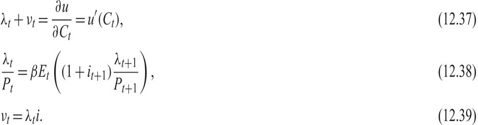
The equilibrium with a price level P^* is locally stable and well defined, but the system is globally indeterminate, because there are an infinite number of adjustment paths that, starting with a price level above P^*, converge to the price level P^** (i.e., infinity). This global indeterminacy is analyzed in figure 12.7.

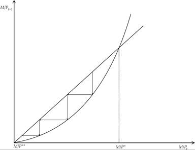
Figure 12.7 Money demand indeterminacy in the Samuelson OLG model.

Note that this global indeterminacy does not arise if the income of the second period is equal to zero (i.e., if the exogenous household income only occurs during the first period of life). In this case, (12.15) simplifies to

This implies a unique equilibrium for the price level.

The second major weakness of this model is that it has no alternative store of value. The only outlet for savings in this model is holding money. However, if there is an alternative asset that pays interest (e.g., bonds or capital), then money would be ostracized from this economy, because its only role is as a store of value, and money does not pay interest. In other words, in the presence of bonds or capital, the demand for money would be equal to zero, because bonds and capital are interest-yielding stores of value, in contrast to money.

Two categories of alternative dynamic general equilibrium models generate a positive demand for money and do not have the weaknesses of the Samuelson OLG model. These two categories, which were first mentioned in chapter 7, are models in which money enters the utility function of households (called money in the utility function models), and models in which economic transactions can only take place through the mediation of money (called cash in advance models).

12.6.2 Money in the Utility Function of a Representative Household

We have already introduced this class of models in the context of the money and growth models in chapter 7. This class of models originates with Patinkin [1956], Sidrauski [1967], and Brock [1974, 1975]. Unlike the Samuelson [1958] OLG model, in this class of models, money can coexist with interest-yielding assets (such as bonds), because it yields direct utility to households, due to its liquidity properties, which facilitate economic transactions.

We will focus on money demand in an endowment economy in which, as in the Samuelson model, real income is exogenous, and there is no capital.

A representative household has an intertemporal expected utility function of the form

where E_t is the mathematical expectations operator, on the basis of information available in period t; C is real consumption of goods and services; M is the quantity of nominal money balances held by the household; P is the price level; and u is a quasi-concave periodic utility function, which is homogeneous of degree one in its two arguments, consumption and real money balances.

The representative household maximizes its intertemporal utility function under the sequence of budget constraints

where Y is the real income of the household, assumed exogenous; T is per capita taxes net of transfers; B is the nominal value of bonds held by the household; and i the nominal interest rate.

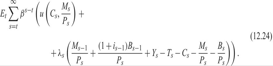
The Lagrange function corresponding to this problem can be written as

The first-order conditions for a maximum with respect to C, B, and M imply

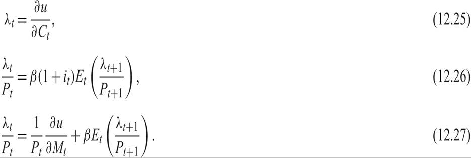
These first-order conditions have the usual interpretations. Equation (12.25) is the static first-order condition, according to which the marginal utility of consumption in any period should equal the “shadow value” of marginal savings λ. Essentially, the household should be indifferent at the margin between consumption and savings.

Equation (12.26) is the dynamic first-order condition that the total expected real return on savings should equal the pure rate of time preference of the household. This can be seen if we take the logarithm of (12.26), which yields

The left-hand side of (12.28) is the total expected real return on savings, taking into account expected inflation and expected capital gains from a change in λ. The right-hand side is the pure rate of time preference of the household, because β = 1/(1 + ρ).

Finally, (12.27) is the dynamic first-order condition that the marginal utility of real money balances equals the difference of the pure rate of time preference from the expected real return of money, taking into account expected inflation and expected capital gains from a change in λ.

From these three first-order conditions, we can derive the demand for money. Assume that the per period utility function takes the form

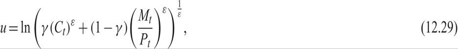
where 1/(1 −ε) is the elasticity of substitution between consumption and real money balances. Under this assumption, using the first-order conditions (12.25)–(12.27), the demand for money function takes the form

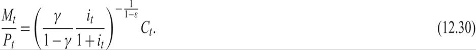
The money demand function depends negatively on the nominal interest rate and positively on total consumption. The negative dependence on the nominal interest rate arises because, with higher nominal interest rates, the opportunity cost of holding money compared to bonds is higher, which reduces the demand for money.

As in the model of Samuelson, for given income, consumption, and nominal interest rate, a one-off increase in the money supply leads to an increase in the price level by the same percentage. As can be seen from (12.30), the neutrality of money holds in this model as well.

12.6.3 Cash in Advance in a Representative Household Model

The basic idea of models in which money is the only means of payment is that to complete any economic transaction, payment must be in the form of money (in particular, cash), which the buyer holds in advance of the completion of the transaction. This idea is due to Clower [1967], and its integration into general equilibrium models leads to a class of models known as cash in advance models.

The restriction that the transaction must be paid with money held in advance imposes a cost of holding money, because otherwise, economic agents could hold an interest-yielding asset, such as bonds.

The cash in advance constraint can take several forms, depending on the assumptions made about the sequencing of transactions. A simple traditional way of expressing this constraint is given by

where M_t−1 is the stock of money accumulated until the end of period t − 1. The problem with this version of the constraint is that someone who enters the economy in period t would not be able to consume at all, because she holds no money.

An alternative hypothesis is that each period consists of two different subperiods. In the first subperiod, agents visit a financial market (say, a bank), where they can swap interest-bearing assets with money, or borrow cash. In the second subperiod, they deal in markets for goods and services, which are liable to the cash in advance constraint (see Lucas [1980, 1982] and Helpman [1981]). This allows the following two-part form of the constraint:

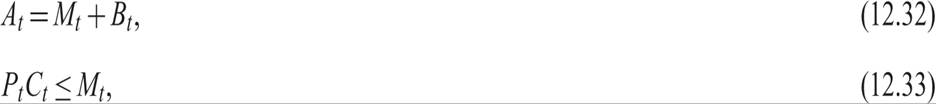
where A is the stock of all nominal assets of the household, M is nominal money balances and B is the value of nominal bonds held by the household.

In the second subperiod, households also receive their exogenous real income Y and pay their taxes (net of transfers) T. As a result, the nominal assets of the household in the beginning of the following period are determined by

The representative household thus maximizes the intertemporal expected utility function

under the sequence of budget constraints (12.34) and the cash in advance constraint (12.33). The Lagrange function is given by

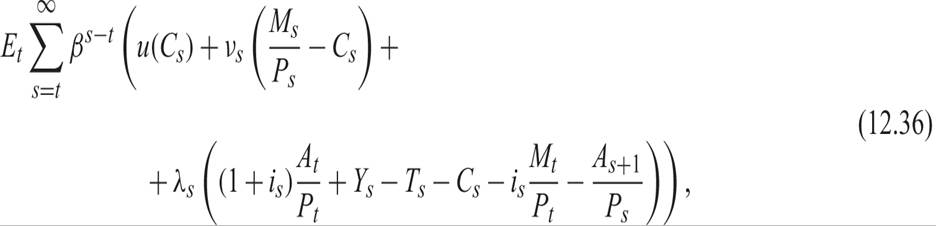
where ν_s and λ_s are the two sequences of Lagrange multipliers.

The first-order conditions for a maximum imply that

The interpretation of these first-order conditions is straightforward. Equation (12.37) is the static first-order condition that on the optimal path, the marginal utility of consumption must be equal to the shadow value of savings λ plus the shadow value of money ν. The shadow value of money results from the restriction that cash in advance is required to buy consumer goods.

Equation (12.38) is the dynamic first-order condition that the total expected real return on savings, including expected inflation and expected capital gains, equals the pure rate of time preference of the household.

Finally, (12.39) is the static first-order condition stipulating that the shadow value of money equals the shadow value of savings times the opportunity cost of holding money, which is none other than the nominal rate (because money pays no interest).

Combining (12.37)–(12.39), one gets

Equation (12.40) is a monetary form of the usual Euler equation for consumption in this model, in which consumption requires money payments in advance. Assuming logarithmic preferences, we have

Under the assumption of logarithmic preference, (12.40) can be written as

The cash in advance constraint implies that

which is a version of the simple quantity equation. Equation (12.43) determines the demand for money function in this model. Monetary neutrality holds in this model as well.

Finally, substituting (12.43) in (12.42), we get

The nominal interest rate depends positively on the pure rate of time preference ρ (which determines β) and the expected rate of change of the money supply (which determines expected inflation).

12.6.4 Cash in Advance in an OLG Model

We now examine the implications for money demand of a cash in advance constraint in a variant of the Samuelson OLG models. In this model, money is both a means of payment and a store of value, unlike the original Samuelson model, in which money was only a store of value.⁹

The household born at the beginning of period t lives for two periods, period t and period t + 1. She receives income Y_t in the first period of life, and consumes in both periods.

The intertemporal utility function of the household is given by

In each period of life, the household is subject to a cash in advance constraint of the form

Aggregate consumption and the money supply in each period are given by

Total assets of households are equal to A, and we assume that young households are born with zero assets. As a result, all assets belong to the old households. For simplicity, assume that taxes T are only paid by young households out of the exogenous income Y.

Given that old households receive no current income, their consumption is equal to their assets:

Note that because of the cash in advance constraint, the old households need to convert their assets into money to purchase consumer goods.

Given that young households hold no assets, they need to borrow at the current interest rate and to convert their loan into money, in order to finance their consumption. As a result, for young households, the following constraints must hold:

The assets of young households at the end of their first period of life will be equal to

From (12.48) and (12.50), it follows that

Introducing (12.51) in the utility function (12.45), we find that young households will choose consumption in their first period of life to maximize

From the first-order conditions for the maximization of (12.52), it follows that

From (12.48) and (12.53), aggregate consumption is given by

From the equilibrium condition in the market for goods and services, we have

Given the cash in advance constraints (12.46), it also follows that

Money demand is thus determined by a simple quantity equation, and the neutrality of money holds in this model as well. Substituting (12.55) in (12.56), we can solve for the price level and the nominal interest rate.

12.7