Nominal and Real Interest Rates and the Money Supply
We next turn to the determinants of the nominal interest rate in the general equilibrium models presented. We will concentrate on three of the models: the model with money in the utility function of a representative household, the representative household model with a cash in advance constraint, and the OLG model with a cash in advance constraint.
In all three models, money demand is positive, even if consumers have the option of holding interest-bearing assets, such as bonds.12.7.1 Money in the Utility Function of a Representative Household
The money demand function in this model is given by (12.30). For simplicity and comparability with the other two models, let us consider the case of logarithmic preferences (ε = 0).
With logarithmic preferences, the first-order conditions for the maximization of the utility function of the representative household are given by
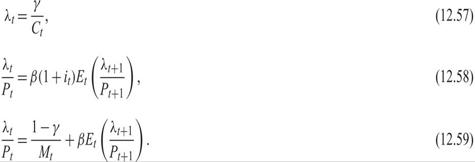
From (12.57) and (12.58) it follows that

Equation (12.60) is the Euler equation for consumption in a representative household economy with money.
From (12.57) and (12.59) it follows that

The rational expectations solution of (12.61) takes the form

Given that Ct = Yt = Y, which is exogenous, (12.62) determines the equilibrium price level as a function of expectations about the future evolution of the money supply.
Substituting (12.62) in the money demand equation (12.30) for ε = 0 and solving for the nominal interest rate yields

The nominal interest rate is determined by the current money supply and expectations about the future development of the money supply, discounted at a rate that depends on the pure rate of time preference of the household.
Assume that the expected growth rate of the money supply is constant and equal to μ. From (12.63), we get
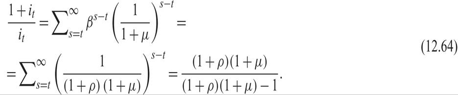
From (12.64), it follows that

Consequently, from (12.65), the higher the growth rate of money supply μ is, the higher will be the nominal interest rate i, as the expected future inflation rate will be higher.
Note that the steady state real interest rate in this model is equal to ρ. For μ = 0, (12.65) implies i = ρ. In this case, because the expected future inflation rate is equal to zero, the nominal interest rate equals the equilibrium real interest rate (i.e., the pure rate of time preference of the representative household).
Note that if μ = −ρ/(1 + ρ) (i.e., if the money supply is reduced at this rate), the nominal interest rate is driven to zero. As argued by Friedman [1969], a zero nominal interest rate has attractive properties and, in the absence of other distortions, leads to the optimum quantity of money, in the sense that the opportunity cost of holding money is equal to its marginal cost of production, which is equal to zero.10
12.7.2 Cash in Advance in a Representative Household Model
In the representative household model in which money demand results from the cash in advance constraint, under the assumption of logarithmic preferences, the nominal interest rate is determined by equation (12.44). Assuming that the growth rate of money supply is equal to μ, (12.44) implies

From (12.66), the nominal interest rate is determined by (12.65), just as in the representative household model with money in the utility function.
Consequently, both representative household models of a monetary economy—the money in the utility function model and the cash in advance model—make identical predictions concerning the determination of nominal and real interest rates.
12.7.3 Cash in Advance in an OLG Model
Finally, we examine the determination of nominal and real interest rates in the Samuelson OLG model with a cash in advance constraint.
From (12.55) and (12.56), it follows that
where Mt −At = PtC1t > 0. The nominal interest rate depends only on the current stock of the money supply and not on its expected future increase.
From (12.67), it follows that

An increase of the current money supply reduces the nominal interest rate, as it increases liquidity in the economy. The effect is similar to the liquidity effect, which we discussed in section 12.3 when analyzing the short-term effects of an increase in the money supply.
12.7.4 The Liquidity Effect in Representative Household Models
The liquidity effect is not so obvious in representative household models. It occurs only as a result of temporary changes in the money supply. This is illustrated by examining the equations for determining the nominal interest rate: (12.63) for the model with money in the utility function and (12.44) for the model with the cash in advance constraint.
Let us confine our analysis to the latter. The nominal interest rate in the cash in advance representative household model is determined by

If there is a temporary increase of the current money supply, which does not affect the expectation of the future money supply, then the impact on the nominal interest rate is given by
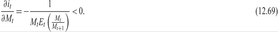
Equation (12.69) shows that there is a liquidity effect for temporary increases in the money supply. Similar properties apply to the model with money in the utility function of a representative household (equation (12.63)).
In contrast, if there is a permanent increase in the money supply, which does not affect the expected ratio between Mt and Mt+1, then this increase has no impact on the nominal interest rate.
There is no liquidity effect for permanent increases in the money supply in representative household models.Finally, for an increase in the money supply that increases the expected ratio between Mt+1 and Mt, then not only is there no liquidity effect, but the opposite occurs (i.e., a positive impact on the nominal interest rate by an increase in the money supply), because an increase in the current money supply signals even higher increases in the future money supply.
For example, assume that the growth rate of the money supply follows a linear first-order, stationary autoregressive stochastic process of the form

where 0 < λ < 1, and εt is a white noise process. It is simple to prove that a positive disturbance εt leads to higher nominal interest rates, because the disturbance causes a temporary increase in the expected ratio between Mt+1 and Mt. Consequently, a positive (albeit temporary) disturbance in the growth rate of the money supply leads to higher nominal interest rates. The reason is that it increases the expected future increase in the money supply and thus expected future inflation. This effect is often referred to in literature as the liquidity puzzle.
The liquidity puzzle is not the only paradoxical property of money demand models of a representative household. A second paradox is the indeterminacy of the price level when the central bank pegs the nominal interest rates instead of the money supply. This has led to large literature on interest rate pegging.
12.8