The Diamond Model

In the Diamond [1965] model, each household lives for only two periods. New households are being born in each period. Thus, in each period, the model assumes the coexistence of two overlapping generations of households: the young, who are in their first period of life, and the old, who are in the second period of life.

5.1.1 Definitions

The definitions of the variables are analogous to those we have used so far. As with the Solow and Ramsey models, we focus on the following set of endogenous variables: Y, aggregate output (or y, output per efficiency unit of labor); K, aggregate (physical) capital stock (or k, capital per efficiency unit of labor); C, aggregate consumption (or c, consumption per efficiency unit of labor); r, real interest rate; and ŵ real wage per worker (or w, real wage per efficiency unit of labor).

The exogenous variables and exogenous parameters in the model are defined as follows: t, time (a discrete exogenous variable); L, population of the young generation (an exogenous variable that depends on time); h, efficiency of labor (an exogenous variable that depends on time); n, rate of growth of population (exogenous parameter); g, rate of technical progress (exogenous parameter); δ, rate of depreciation of capital (exogenous parameter); ρ, pure rate of time preference of households (exogenous parameter); and θ, inverse of the elasticity of intertemporal substitution.

5.1.2 The Production Function

The technology of production is described by a neoclassical production function, analogous to the one we assumed in the Solow and Ramsey models. The production function has all the properties of the neoclassical production function assumed in the Solow model.

Because of the assumption of constant returns to scale, the production function can be rewritten as

where y = Y/hL is output per efficiency unit of labor, k = K/hL is capital per efficiency unit of labor, and f(k) = F(k, 1) is the production function per efficiency unit of labor.

5.1.3 The Intertemporal Utility Function of Households

In period t, L_t households are being born, and population grows at an exogenous rate n:

The young (i.e., those in the first period of life) work, while the old (those in the second period of life) do not. Thus, each household supplies a unit of labor when young and allocates labor income between consumption of the first period and savings. In the second period of life, old households consume their savings plus the interest on their savings. Thus, each generation chooses savings to solve a Fisherian problem.

The utility function of a household born in period t is defined by

where 0 < θ < 1, ρ > −1, and c_1t, c_2t+1 denote consumption in the first and second period of life, respectively. Equation (5.4) is the constant elasticity of intertemporal substitution utility function, known to us from chapter 2. Here, θ is the coefficient of constant relative risk aversion, and 1/θ is the constant elasticity of intertemporal substitution of consumption.

5.1.4 Markets and the Behavior of Households

Production takes place by many competitive firms, each with a production function like (5.1).

where Af′(k_t) is the marginal product of capital.

Each young household allocates its labor income w_th_t between consumption and savings. As a result, the capital stock of period t + 1 is equal to the aggregate savings of period t:

This capital stock is combined in production with the labor supplied by the generation born in period t + 1, and the economy continues from period to period.

In the second period of life, the household born in period t consumes all its interest income plus the savings it has accumulated in the first period of life. Thus, consumption in the second period of life of a household born in period t is given by

Maximizing (5.4) under the budget constraint (5.8) and rearranging the first-order conditions, we get the following expression for the ratio of consumption in the two periods:

which is the first-order condition of the Fisher model of chapter 2 and is analogous to the Euler equation for consumption in the Ramsey model analyzed in chapter 4. Consumption in the second period of life is higher or lower than consumption in the first period of life, depending on whether the real interest rate exceeds or falls short of the pure rate of time preference. The elasticity of intertemporal substitution of consumption determines the elasticity of the effect.

Using (5.8) and (5.9) to solve for c_1t, we get

Young households consume a share of their labor income that depends on their preferences and the real interest rate. We can rewrite (5.9) as

where s is the savings rate of young households, defined as

Equation (5.11) suggests that the savings rate is a positive function of the real interest rate r only if θ is lower than unity (i.e., if the elasticity of intertemporal substitution of consumption 1/θ is higher than unity). Only in this case does the substitution effect dominate the negative income effect. If θ is greater than unity, the savings rate is a negative function of r, as the income effect dominates. In the special case that θ is equal to one (i.e., logarithmic preferences), the savings rate is independent of the real interest rate and is equal to 1/(2+ρ).⁴

We can now aggregate the savings behavior of the two overlapping generations and determine capital accumulation and the dynamic adjustment of this economy.

5.1.5 Capital Accumulation and the Dynamic Adjustment of the Economy

The aggregate capital stock in each period is equal to the savings of young households of the previous period, because the old households of the previous period consumed all their capital and the young households of the current period own no capital. Thus, we have

Expressing (5.12) in efficiency units of labor, dividing by h_t+1L_t+1, we get

Substituting for r and w from (5.5) and (5.6) yields

This equation determines the dynamic behavior of capital per efficiency unit of labor.

As with previous models, the first question that arises is whether a steady state equilibrium point k^* exists, and, if it does, whether the economy converges to this steady state. Equation (5.14) is a nonlinear first-order difference equation in the capital stock per efficiency unit of labor. Because of nonlinearity, there is the possibility of multiple equilibria. Figure 5.1 highlights this possibility for a general form of the production function.

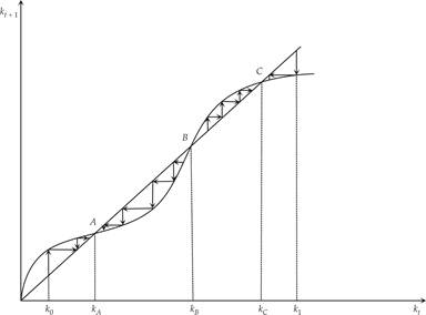
Figure 5.1 Multiple equilibria in the Diamond model.

The 45° line is the locus of equilibrium points, for which,

The nonlinear curve is the geometric version of a possible general form of (5.14). As shown in figure 5.1, there are at least three possible equilibria for this general form of the curve: A, B, and C. Of these, A and C are locally stable, and B is unstable. Which equilibrium is reached by the economy depends on initial conditions.

If the initial capital per efficiency unit of labor is equal to k₀, then the economy will converge to equilibrium A. If the initial capital per efficiency unit of labor is higher than B, then the economy will converge to C. Thus, at least two potential stable equilibria exist, depending on initial conditions. There is no guarantee that the economy will converge to a unique balanced growth path as in the Solow and Ramsey models.

Consequently, the Diamond model differs from the models examined so far, in that it can result in multiple balanced growth paths in its general form. There is no unique balanced growth path toward which an economy will converge regardless of initial conditions.

As illustrated in figure 5.1, an economy with a low initial capital stock will converge to a balanced growth path like A, which is characterized by low capital and output per efficiency unit of labor. Per capita income in the balanced growth path will therefore be lower than in an economy that has a high initial capital stock (greater than that corresponding to point B) and converges to a balanced growth path like C, which is characterized by a higher capital stock and output per efficiency unit of labor.⁵

5.1.6 A Simplified Diamond Model with Logarithmic Preferences and Cobb-Douglas Technology

The Diamond model can be simplified significantly if one assumes logarithmic preferences (θ = 1) and a Cobb-Douglas production function (Af(k) = Ak^α). Then (5.6) and (5.12) simplify to

In this case, the real wage is a constant share of output, and the savings rate is independent of the real interest rate. Substituting in (5.13), the adjustment equation for capital per efficiency unit of labor takes the form

One can show, as in figure 5.2, that in this case, a unique balanced growth path exists, because of the constant savings rate and the properties of the Cobb-Douglas production function. The Diamond economy converges to this unique balanced growth path k^* independently of the initial conditions, as long as the initial capital stock is positive.

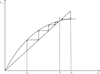
Figure 5.2 Unique balanced growth path in the simplified Diamond model.

The properties of this simplified Diamond model are analogous to those of the Solow and Ramsey models. On the unique balanced growth path, the savings rate is constant. Output, consumption, and the real wage per worker grow at a rate g, while the capital output ratio and the real interest rate are constant.

Figure 5.3 examines the impact of a previously unanticipated permanent increase in the pure rate of time preference in the simplified Diamond model. This has the effect of reducing the savings of the young generation, which leads to a lower level of capital in the following period compared with the initial equilibrium level k^*. This decline sets in motion a process of capital decumulation until the economy converges to the new equilibrium k^**, in which the capital stock per efficiency unit of labor is lower. Consequently, as in the Ramsey model, an increase in the pure rate of time preference in the simplified Diamond model eventually leads to an equilibrium with a lower capital stock and real output per efficiency unit of labor.

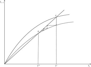
Figure 5.3 Effects of a permanent rise in the pure rate of time preference.

A decrease in the pure rate of time preference has the opposite effects. In the new balanced growth path, both consumption and capital per efficiency unit of labor will be higher. Consumption will initially fall; the economy will begin accumulating additional capital; and on the new balanced growth path, the economy will end up with a higher capital stock and real output and income per efficiency unit of labor.

As in the representative household model, the pure rate of time preference is a key determinant of the savings rate. The higher it is, the smaller will be the savings of the young as well as the overall savings rate. Recall that in this model, it is only the young that save, as the old have negative savings, because they consume both their current income and their capital.

An increase in the population growth rate n or an increase in the rate of exogenous technical progress g has similar effects to an increase in the pure rate of time preference, leading to a lower capital stock and real output and income per efficiency unit of labor. The analysis would be similar to the analysis in figure 5.3.

Note that, with regard to the rate of growth of population, the Diamond OLG model has different predictions than the Ramsey representative household model. In the Diamond model, an increase in the rate of population growth, which leads to an increase in steady state investment, is not matched by a equal increase in savings through an adjustment of the savings rate. This is because current generations do not internalize the welfare of future generations, as in the case with the representative household model. Hence, an increase in the rate of population growth leads to a decline in the capital stock, so that steady state investment adjusts to savings. This is a major difference between representative household and OLG models and is something that we shall also encounter in chapter 6 and 7, when we discuss the effects of government debt or monetary policy in growth models.

Figure 5.4 analyzes the impact of a previously unanticipated permanent rise in total factor productivity A. This causes an immediate increase in income and savings for a given capital stock per efficiency unit of labor. The rise in aggregate savings leads to capital accumulation, until the capital stock approaches its new higher steady state value at k^**. Consequently, after a permanent increase in total factor productivity, the economy converges to a new balanced growth path, with higher steady state capital, output, and income per efficiency unit of labor.

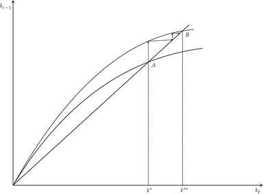
Figure 5.4 Effects of a permanent rise in total factor productivity.

5.1.7 The Speed of Adjustment in the Simplified Diamond Model

As for the Solow and Ramsey models, it is worth exploring the quantitative as well as the qualitative properties of the simplified Diamond model. From (5.15), the economy is on the balanced growth path k^* when

Solving for the steady state capital per efficiency unit of labor k^*, we get

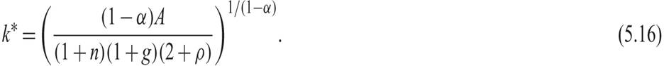
From the production function, steady state output per efficiency unit of labor y^* is then equal to

Equation (5.17) determines output per efficiency unit of labor on the balanced growth path and its dependence on technological and population growth parameters (such as A, α, g, and n), as well as on parameters of the preferences of households (such as ρ). From estimates of the values of the various parameters, we can get quantitative estimates for the long-term effects of various changes in the parameters on steady state output. Note that because in this model the length of the time period equals half the life expectancy of an adult, the choice of parameters should take account of this fact. For example, n must be calculated not as the annual rate of population increase but as the population growth rate over 30 years. Similar choices have to be made for other parameters, such as g and ρ.

To find the speed of adjustment toward the balanced growth path, we take a linear approximation of (5.15) around the steady state capital stock, k = k^*. This is given by

From (5.15) and (5.17) we have that

The speed of adjustment therefore depends on only one parameter, the exponent (share) of capital in the Cobb-Douglas production function. If α equals 1/3, then in each period, the capital stock per efficiency unit of labor moves 2/3 of the distance that separates it from the value corresponding to the balanced growth path. If the period is 30 years, this amounts to about 2% per year.

Recall that in this model, under the assumption of logarithmic preferences, the savings rate is constant only for the young generation. The negative savings of the old generation are not a constant percentage of its income but instead increase in absolute terms as the capital stock per efficiency unit of labor increases. This is because of diminishing returns to capital accumulation that reduce the old generation’s interest income. As a result, in the simplified Diamond model, total savings as a percentage of total income (the aggregate savings rate) are a negative function of capital per efficiency unit of labor k. The same applies to the representative household model with a Cobb-Douglas production function and logarithmic preferences.

5.1.8 Welfare Implications of the Diamond Model and the Possibility of Dynamic Inefficiency

The greatest difference between the representative household model and the OLG model is perhaps related to its welfare implications and the efficiency of the equilibrium. We saw that in the Ramsey model, competitive equilibrium leads to the maximization of welfare of the representative household. In OLG models, a representative household does not exist, and therefore it is not clear how we would evaluate the welfare implications of the competitive equilibrium. If we define social welfare as a weighted average of the welfare of the different generations, there is no reason to expect that the competitive equilibrium would lead to the maximization of that weighted average.

The minimum efficiency criterion we have in economics is Pareto efficiency, which states that it is impossible to make someone better off without making somebody else worse off. But even the simplified Diamond model does not necessarily satisfy this criterion. Theoretically, the capital stock on the balanced growth path can exceed that which satisfies Pareto efficiency and corresponds to the golden rule. Thus, the Diamond model may even be characterized by dynamic inefficiency. Therefore, a social planner could, if the economy ends up with more capital than the golden rule, theoretically increase the level of consumption (and therefore the level of welfare of all generations) by reducing savings and the aggregate capital stock.

To see how this possibility can arise, we focus on the simplified Diamond model with logarithmic preferences and a Cobb-Douglas production function.

The steady state capital stock is given by (5.16). Its marginal product is given by

On the balanced growth path, the capital stock that satisfies the golden rule has a marginal product equal to the growth rate. It must satisfy

where GR stands for the golden rule value.

For a sufficiently small α, the marginal product of the steady state capital stock, as given by (5.20), could be smaller than the marginal product corresponding to the golden rule, which is given by (5.21). This would mean that the steady state capital stock is higher than the golden rule capital stock. As a result, a social planner could increase the current consumption and welfare of all generations by reducing savings and the steady state capital stock to the level corresponding to the golden rule. As we have already discussed in the case of the Solow model, a steady state in which the marginal product of capital is lower than the long-term growth rate of the economy results in dynamic inefficiency.

How likely is dynamic inefficiency in the case of the simplified Diamond model? The answer is largely an empirical matter. Staying in the confines of the model, let us assume that the share of capital in total income α is equal to 1/3, the annual population growth rate n is 1%, the annual rate of technical progress g is 2%, and that the annual pure rate of time preference ρ is 2%. These are the empirical assumptions that we have made so far. Also assume that the time period in the Diamond model is equal to 30 years. Thus, over 30 years, n = 0.348, g = 0.811, and ρ = 0.811.

Under these assumptions, the marginal product of steady state capital from (5.20) is equal to 4.44. From (5.21), the marginal product of the capital stock that corresponds to the golden rule is equal to 1.44. Thus, based on these empirical estimates of the parameters, the possibility of dynamic inefficiency does not arise in the simplified Diamond model. With the assumptions about n, g, and ρ that we have made, the share of capital should be lower than 1/6 instead of 1/3 for the possibility of dynamic inefficiency to arise.

In any case, when Abel et al. [1989] explored the possibility of dynamic inefficiency empirically for the US economy and six other developed economies, they concluded that the marginal product of capital comfortably exceeds the long-run growth rate, a finding that rules out the possibility of dynamic inefficiency for the developed economies.

On the basis of these observations and the available empirical evidence, the possibility of dynamic inefficiency, although theoretically interesting, does not seem likely. Besides, it would mean that there is excess saving, which is in contrast with other empirical features of developed market economies, such as current account deficits in many of them.

5.1.9 Dynamic Simulations of a Calibrated Diamond Model

To further investigate the process of dynamic adjustment characterizing the simplified Diamond model, we can simulate, for specific calibrated values of the parameters of the model, the process of dynamic adjustment from one balanced growth path to another, when there is an exogenous permanent change in specific parameters. As for the Ramsey model, let us shall concentrate on changes in the pure rate of time preference and total factor productivity. But we shall also report on the effects of a rise in the rate of growth of population, which only affects per capita consumption and not per capita output or capital in the Ramsey model.

In the simulation, it is assumed that the production function has the usual Cobb-Douglas form, Af(k) = Ak^α, and that the intertemporal elasticity of substitution in consumption is equal to unity. The evolution of total private consumption can be derived from the consumption functions of young and old households. The evolution of the real interest rate and real wages per efficiency unit of labor can be derived from the usual marginal productivity conditions (5.5) and (5.6) for a Cobb-Douglas production function.

The model was simulated for the following parameter values: A = 1, α = 1/3, θ = 1, ρ = 0.811, n = 0.348, g = 0.811, δ = 1.427. Unlike the previous models, which assumed that the time period is a calendar year, here the time period is 30 years, the half-life of a generation. An annual rate of 1% is converted into a 30-year rate of 34.8%, an annual rate of 2% is converted into a 30-year rate of 81.1%, and an annual rate of 3% is converted into a 30-year rate of 142.7%.

We consider two alternative scenarios: a permanent increase in the pure rate of time preference of households ρ by 1% and a permanent increase in total factor productivity A by 1%. The results of the simulations are presented in figures 5.5 and 5.6.

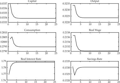
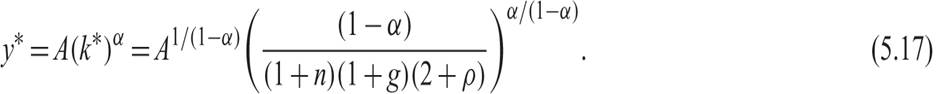
Figure 5.5 Impulse response functions of the Diamond model for a permanent rise in the pure rate of time preference of 1%.

Figure 5.6 Impulse response functions of the Diamond model, for a permanent rise in total factor productivity of 1%.

In figure 5.5, the economy is on its original balanced growth path, and after period 1, the pure rate of time preference of the young generation ρ rises by 1%, from 0.811 to 0.819, where it remains thereafter. This increase leads directly to an increase in consumption of the young, a decline in the savings rate, a gradual decumulation of capital, a gradual decline in output and real wages, and a gradual increase in the real interest rate. The reason for the decline in real wages is the gradual reduction of the marginal product of labor; the reason for the increasing real interest rate is the gradual increase in the marginal product of capital. Both trends are caused by the declining capital stock. The economy gradually converges to a new balanced growth path. On this new path, capital per efficiency unit of labor is lower by about 0.9% compared to the original path, output and real wages are lower by 0.3%, consumption is lower by 0.3%, and the real interest rate has increased by 1.1%. The steady state savings rate for the economy as a whole, which is endogenous in this model, has declined slightly, from 13.31% to 13.30%. This drop is due to the slight fall in the savings rate of the young. Recall that the savings rate of the young, with logarithmic preferences, is independent of the real interest rate and only depends on the pure rate of time preference, as it is equal to 1/(2 + ρ).

A similar simulation has also been conducted, in which the rate of population growth n rises by 1% (from 0.348 to 0.351). The dynamic path is similar to the simulation for the pure rate of time preference, but the steady state effects are smaller. Per capita output and real wages fall by only 0.1%, about one-third of the effects of a similar rise in the pure rate of time preference. Per capita capital falls by 0.4% and per capita consumption by 0.2%. The effects are quantitatively smaller, because there is no additional negative effect through the decline in the savings rate of the young generation, which occurs for the case with the decline in the pure rate of time preference.

In the simulation shown in figure 5.6, the economy is on its original balanced growth path, and after period 1, total factor productivity A rises permanently by 1%, from 1 to 1.01. This increase leads immediately to an increase in production, consumption, savings, and the marginal product of both labor (real wage) and capital (real interest rate). The increase in savings causes a gradual accumulation of capital, which leads to a further gradual increase in production, consumption, and the real wage, and a gradual decline in the real interest rate. The reason for the declining real interest rate is the gradual reduction of the marginal product of capital caused by the accumulation of capital. The economy gradually converges to a new balanced growth path. On this new path, capital per efficiency unit of labor is increased by about 1.5%; output, consumption, and real wages have also increased by 1.5%; whereas the real interest rate has returned to very near its original equilibrium. An increase in productivity by 1% leads to an increase in real output by 1.5% (i.e., more than 1%) because higher total productivity causes a temporary increase in the savings rate and capital accumulation, which causes secondary increases in the capital stock, real output, consumption, and real wages.

As we can see from these simulations, the dynamic behavior of the simplified Diamond OLG model is qualitatively similar to that of the Ramsey model of a representative household. Although the models differ in the specific assumptions they make about the determination of aggregate savings, they result in qualitatively similar properties regarding the process of adjustment toward the balanced growth path. In addition, despite the prediction that the savings rate is not constant along the adjustment path, as assumed in the Solow model, in all other respects, the predictions of the Diamond and Ramsey models about the adjustment path are very similar to the predictions of the Solow model.

However, the Diamond model has one important difference from the representative household model. The rate of population growth affects the steady state per capita output and capital stock negatively, as in the Solow model with an exogenous savings rate. The reason is that current generations do not take into account the welfare of future generations, and thus they do not adjust their savings by enough to allow for a higher population growth.

5.2