The Blanchard-Weil Model

We now turn to an alternative OLG model, the model of Blanchard [1985] and Weil [1989], also known as the model of perpetual youth.⁶

In the Blanchard-Weil model, it is assumed that new households are being born continuously, with each household having an infinite time horizon.

In the original version of this model by Blanchard [1985], at any instant there is a constant probability of death, which is independent of the age of households. In the model of Weil [1989], the probability of death is zero (i.e., households not only have an infinite time horizon but discount the future only by using the pure rate of time preference and not the probability of death).

What emerges from the model of perpetual youth is that the main differences between the predictions of OLG models and representative household models result from differences in the age of different households and not the possibility of death.⁸

Technology and market structure in this model is similar to the previous models we have analyzed so far. We have competitive markets and a neoclassical production function with constant returns to scale.

5.2.1 Definitions

The definitions of the variables are analogous to those we have used so far. As with the Solow, Ramsey, and Diamond models, we shall focus on the following set of endogenous variables: Y, aggregate output (or y, output per efficiency unit of labor); K, aggregate (physical) capital stock (or k, capital per efficiency unit of labor); C aggregate consumption (or c, consumption per efficiency unit of labor); r real interest rate; and ŵ, real wage per worker (or w, real wage per efficiency unit of labor).

The exogenous variables and exogenous parameters in the model are defined as follows: t, time (a continuous exogenous variable); L, total population and employment (an exogenous variable that depends on time); h, efficiency of labor (an exogenous variable that depends on time); n, rate of growth of population (exogenous parameter); g, rate of technical progress (exogenous parameter); δ, rate of depreciation of capital (exogenous parameter); and ρ, pure rate of time preference of households (exogenous parameter).

With regard to L and h, we also assume that

5.2.2 The Production Function

Production takes place on the basis of technological possibilities described by a neoclassical production function, similar to the one assumed in the Solow, Ramsey, and Diamond models:

The production function is characterized by constant returns to scale, so it can be written as

where y = Y/hL, output per efficiency unit of labor; k = K/hL, capital stock per efficiency unit of labor; and f(k) = F(k, 1), production function per efficiency unit of labor.

5.2.3 The Intertemporal Utility Function of Households and Household Consumption

Following Weil [1989], let us assume that households have an infinite time horizon (i.e., that they are dynasties) but differ in their birth dates. Each instant, nL new households are born. New households have no connection with old households whatsoever. The typical household born at time j chooses the path of its current and future consumption to maximize the intertemporal utility function:

where c( j, t) is consumption of household j at instant t, u is the instantaneous concave utility function, and ρ is the pure rate of time preference.

Following Blanchard [1985] and Weil [1989], we shall assume that the instantaneous utility function is logarithmic. This is equivalent to assuming a unitary elasticity of intertemporal substitution of consumption:

All households have a constant number of members (assumed to be equal to one), with each supplying one unit of labor. All households, irrespective of their date of birth, can borrow and lend freely at the market-determined real interest rate r.

Moreover, we assume that there exist a large number of competitive firms, each with a production function similar to (5.22). Markets are competitive, and therefore the real interest rate and the real wage are defined by the marginal productivity conditions

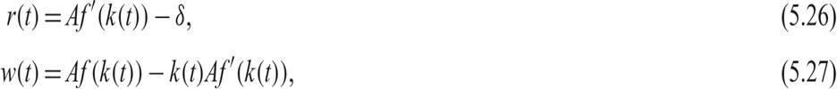
where f′(k) is the marginal product of capital. Therefore, household j maximizes (5.24) under the constraint

where k( j, j) = 0.

From the first-order conditions for a maximum, we can derive the Euler equation for consumption of household j:

Integrating (5.29) over time and using the fact that the present value of consumption is equal to initial assets plus the present value of labor income for all households, we get the following consumption function:

alt=eq5-30.png>

where

Here, Ŵ(t) is the present value at time t of labor income (human capital). From (5.31), we can confirm that the present value of labor income is the same for all households, irrespective of their birth date, because the real wage is the same for all households, as is labor efficiency, and all households supply one unit of labor per instant.

From (5.30), we can see that the average and marginal propensity to consume wealth (the sum of nonhuman and human capital) is the same for all households and is equal to the pure rate of time preference. This is a consequence of logarithmic preferences and the assumption that there is no population growth in households.⁹

5.2.4 Aggregation across Generations

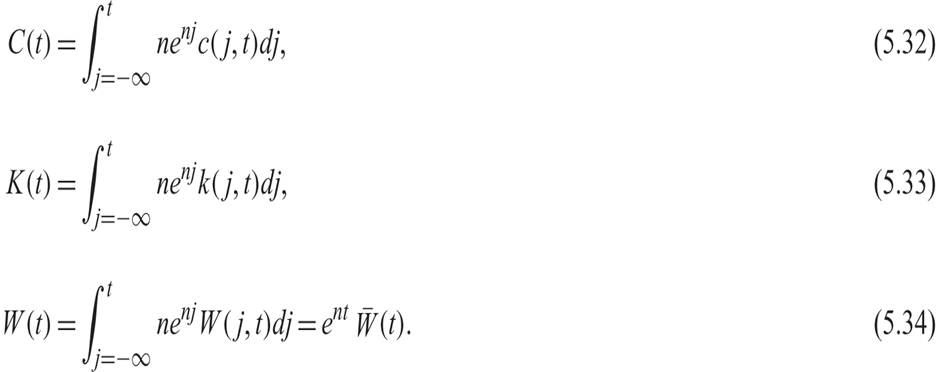
The aggregate variables C(t), K(t), and W(t) are determined by the integral of the variables that correspond to every generation of households at time t (i.e., for every j ≤ t). For every generation j, its size, equal to ne^nj, is taken into account. Obviously, younger generations are more numerous than older generations. As a result, aggregate consumption and aggregate physical and human capital are given by

From (5.30) and (5.32), it follows that

and (5.35) gives

From (5.28) and (5.33), it follows that

and from (5.34), we have

Finally, (5.35) to (5.38) yield

Equation (5.39) describes the evolution of aggregate consumption over time. To the extent that the real interest rate exceeds the pure rate of time preference, all households accumulate capital, which leads to an increase in their consumption. In addition, because of the addition of new households at rate n, aggregate consumption increases because of the additional consumption of these households.

5.2.5 The Model in Terms of Efficiency Units of Labor

Consumption and the capital stock per efficiency unit of labor are defined as

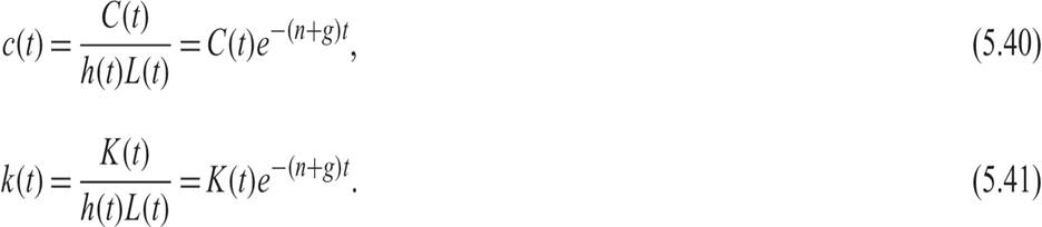
From (5.40) and (5.41), it follows that

Using (5.26) to substitute for the real interest rate in (5.42), consumption per efficiency unit of capital evolves according to

From (5.37) and (5.41), and using the constant return to scale property of the production function and the marginal productivity conditions (5.26) and (5.27) for the real interest rate and the real wage, we get the following accumulation equation for capital per efficiency unit of labor:

This is the usual accumulation equation, which defines the change in the capital stock per efficiency unit of labor as the difference between savings and steady state investment (n + g + δ)k.

We can now use (5.43) and (5.44) to analyze both the balanced growth path and the process of adjustment toward the balanced growth path.

5.2.6 The Balanced Growth Path and the Adjustment Path

We now analyze the balanced growth path and the adjustment path using a phase diagram analogous to that used for the Ramsey model. On the balanced growth path, we have that

From (5.43), the condition for constant consumption per efficiency unit of labor is given by

From (5.44), the condition for constant capital per efficiency unit of labor is given by

The balanced growth path (steady state) is defined by the simultaneous satisfaction of conditions (5.45) and (5.46).

The geometric depiction of both the balanced growth path and the adjustment path in this model is presented in figure 5.7. The balanced growth path is determined at the point (k^*, c^*), where (5.45) and (5.46) are simultaneously satisfied. In the figure, (5.45) is depicted by the curve (the steady state consumption curve), and (5.46) is depicted by the curve (the steady state capital curve). The balanced growth path is a saddle point, and only one adjustment path leads to the balanced growth path. All other paths do not satisfy the relevant transversality condition.

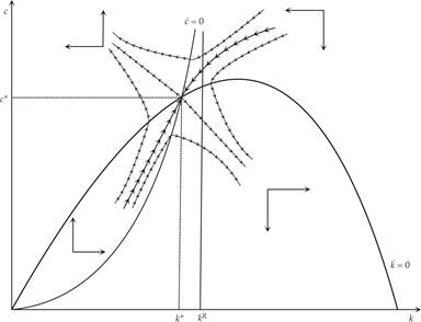
Figure 5.7 The balanced growth path and the adjustment path for the Blanchard-Weil model.

Note that the balanced growth path lies to the left of the balanced growth path that would prevail in the case of a representative household (k^R in figure 5.7). In the steady state of the model of overlapping generations with perpetual youth, both the capital stock and the level of consumption (per efficiency unit of labor) are lower than the values corresponding to the modified golden rule. This is because current generations do not internalize the welfare of future generations, and they end up saving less than a representative household that takes the welfare of future generations into account. For this reason, and despite competitive markets, the balanced growth path in the model of perpetual youth is not socially efficient in the sense of maximizing social welfare. Redistributing capital to favor the new generations would result in higher consumption and output per efficiency unit of labor. However, the possibility of dynamic inefficiency does not arise in this model. The capital stock cannot be higher than the level corresponding to the golden rule.

As in the Ramsey model, a unique saddle path leads to the steady state. Because consumption is not a predetermined variable but the capital stock is, from any initial position, consumption will directly adjust to put the economy on the unique saddle path leading to the steady state. To the left of k^*, consumption is lower than its steady state value, and the economy accumulates capital. During this process, capital and consumption per efficiency unit of labor are increasing. The opposite occurs if the initial capital stock is to the right of the steady state capital stock. Both the capital stock and consumption per efficiency unit of labor are higher than in the steady state and are decreasing on the unique saddle path.

Exercise 5.1 Assuming a Cobb-Douglas production function, derive the steady state of the Blanchard-Weil OLG model from the system of differential equations (5.43) and (5.44). Discuss the determinants of all steady state variables. Also analyze the stability of the system by linearizing the system around the steady state. Compare the steady state of the Blachard-Weil OLG model to that corresponding to the comparable representative household model. What determines the growth rate of per capita output, consumption, and real wages in the steady state?

Figure 5.8 shows the effects of an increase in the pure rate of time preference of households. An increase in pure rate of time preference leads to a shift of the steady state consumption function to the left. At the new equilibrium (c^**, k^**), both consumption and the capital stock per efficiency unit of labor will be lower. When the shift occurs, consumption increases from c^* to c₀ and puts the economy on the saddle path corresponding to the new balanced growth path. Savings are lower than equilibrium investment, and the economy starts to decumulate capital, gradually adapting to the new balanced growth path, with lower consumption and capital per efficiency unit of labor.

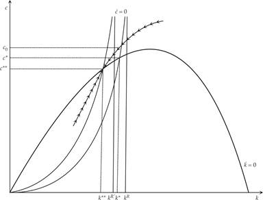
Figure 5.8 Short- and long-run effects of an increase in the pure rate of time preference in the Blanchard-Weil model.

A decrease in the pure rate of time preference has the opposite effect. At the new equilibrium, both consumption and capital will be higher. When the shift occurs, consumption decreases, the economy begins to accumulate additional capital, and it gradually adjusts to the new balanced growth path with higher capital and consumption per efficiency unit of labor.

We thus see that in this model, the pure rate of time preference is a key factor determining savings behavior and the balanced growth path. The higher it is, the less households of all generations will save, as they prefer more utility from consumption today relative to utility from future consumption.

The short- and long-run effects of a previously unanticipated permanent increase in the rate of population growth n are analyzed in figure 5.9. The Blanchard-Weil OLG model differs from the Ramsey representative household model in the effects of a change in population growth n. In the Ramsey model, population growth occurs in the representative household and is internalized by the savings behavior of the representative household. Thus, as already shown, population growth affects only consumption and not capital per effective unit of labor. In the Blanchard-Weil model, population growth is external to existing households, as it takes the form of additional households. Therefore, population growth is not internalized. As a result, an increase in population growth results in an insufficient increase in savings, which results in the decumulation of capital. On the new balanced growth path, both consumption and the capital stock go down as a result of higher population growth. In this respect, the Blanchard-Weil model resembles the Solow and Diamond models, in which population growth has a negative impact on per capita income.

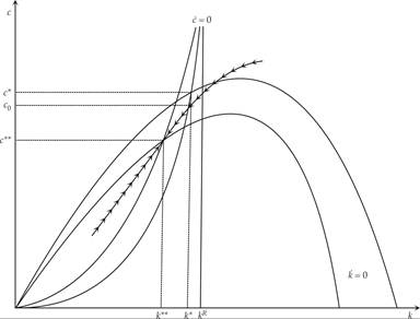
Figure 5.9 Short- and long-run effects of an increase in the rate of population growth in the Blanchard-Weil model.

A rise in population growth shifts the steady state consumption curve up and the steady state capital accumulation locus down. In the new balanced growth path, both consumption and the capital stock per efficiency unit of labor are lower. When the shift occurs, consumption declines, but not by enough to prevent the decumulation of capital, as in the case of the representative household model. The reason is that current generations do not internalize the welfare of future generations. Thus, the economy adjusts along the new saddle path, on which savings are lower than steady state investment. The economy continues to decumulate capital and gradually adapts toward the new balanced growth path (c^**, k^**), with lower consumption and capital per efficiency unit of labor.

5.3